Department of Economics University of Southampton Southampton SO17 1BJ UK
Discussion Papers in
Economics and Econometrics
2000
The Quality of Life in England and Wales
¤Sylaja Srinivasan
Geo¤ Stewart
Department of Economics
University of Southampton
August 14, 2000
Abstract
Local amenities play an important role in determining where we choose to live and our overall quality of life. In many cases, however, amenities do not have prices and will therefore be underprovided by the market. In this paper, we use individual and county level data for England and Wales to estimate implicit amenity prices and to calculate an index of quality of life for each county. Among our …ndings is a large negative price on air pollution. The range in quality of life across counties is estimated to be in excess of two thousand pounds per year.
JEL Classification: I31, R1
Keywords: Quality of Life index, amenities, hedonic prices.
Address for Correspondence: Geo¤ Stewart, Department of Economics, University
of Southampton, High…eld, Southampton SO17 1BJ, U.K. Tel: +44 (0)23 8059 2520; Fax: +44 (0)23 8059 3858; e-mail: gs@soton.ac.uk
¤We wish to thank Sujoy Mukerji, Raymond O’Brien and Jackline Wahba for helpful comments. We
1 Introduction
Our quality of life depends on where we live. But just how much value do we put on a good
location? And what are the factors that determine the attractiveness of an area? These
questions, interesting in themselves, derive added importance from the fact that a number of
potentially important amenities - for instance, clean air - do not have prices and will therefore
be underprovided by the market. Furthermore, the absence of prices creates di¢culties for the
design of policies to deal with this ine¢ciency; indeed, to the extent that policy tends to focus
on variables that are relatively easy to measure, government intervention may actually have
an adverse impact on amenity provision. In the UK, the government itself has recently argued
that various dimensions of the quality of life have su¤ered as a consequence of the reliance on
GDP as a measure of economic success. Its proposed response incorporates a commitment to
publish data on some 150 quality of life indicators, ranging from average life expectancy to
populations of wild birds.1 This clearly marks an important …rst step in tackling the problem.
However, to address the inevitable policy trade-o¤s it is necessary to consider how much weight
people put on each of the contributors to their quality of life; ideally these preferences would
be expressed in monetary terms. A set of weights would also be required to aggregate the
individual elements into an overall measure of quality of life.
In a seminal contribution to the theoretical literature on the quality of life, Roback (1982)
showed how the locational decisions of individuals and …rms lead to an equilibrium in which
di¤erences in amenity levels are re‡ected in wage and house price di¤erentials, and that these
di¤erentials can then be used to estimate monetary valuations - ‘implicit prices’ - for each
amenity. Thus the relative value of each component of quality of life is inferred from
individ-uals’ actual decisions in labour and housing markets. In this paper, we apply Roback’s model
to county level data for England and Wales. Among our …ndings are a large negative price
on air pollution and, perhaps surprisingly, a positive price on population density. The set of
implicit prices is then used to calculate an index of the overall quality of life in each of the
counties. This points to considerable variation across England and Wales: for the
tative household, the di¤erence in quality of life between the top-ranked and bottom-ranked
county is estimated to be well in excess of two thousand pounds per year.
Amenity pricing and the measurement of quality of life has attracted considerable interest
in the US. Early empirical work derived implicit amenity prices from data on either residential
property values or wages. For example, Ridker and Henning (1967) estimated that variations
in air pollution levels explained 1.2 per cent of the variance in house prices in St. Louis. More
ambitiously, Nordhaus and Tobin (1972) used estimates of implicit prices based on wage data
to calculate the cost of urbanisation to the entire US economy. The …rst study to construct a
quality of life ranking on the basis of amenity prices was Rosen (1979). He used census data
on wages and characteristics of almost nine thousand individuals to estimate implicit prices
for pollution, crime, climate, and measures of crowding and labour market conditions. These
prices were then combined with the quantities of each amenity to produce quality of life index
values for …fteen major US cities.
A major theoretical contribution to the literature was provided by Roback’s (1982) general
equilibrium model of individual and …rm location. Drawing upon Rosen (1974), she showed
how wages and land prices are simultaneously determined by the location decisions of workers
and …rms and thatboth wage and rent gradients are required in order to determine the implicit price of an amenity. Roback applied her model to data on individuals’ wages and average land
prices to produce estimates of implicit amenity prices and a ranking of twenty of the largest
US cities. Using the same methodology, but more detailed data, Blomquist, Berger and
Hoehn (1988) examined the quality of life in 253 US urban counties in 1980. Their results
suggest strongly that compensation for amenity e¤ects occurs in both labour and housing
markets. Moreover, the amounts involved were large: the estimated di¤erence in quality of
life between the top-ranked county (Pueblo) and the bottom-ranked (St. Louis City) was
$5146 per household per year in 1980. Subsequent empirical work in the US has extended the
analysis in various directions. For example, Gyourko and Tracy (1991) introduced the e¤ect
of local …scal conditions, and Clark and Nieves (1995) incorporated detailed data on nuclear
plants, petrochemical re…neries and other noxious facilities.
In Britain, empirical work has been hampered by data limitations. The only previous
estimates of amenity values using the Roback framework are those of Maddison (1997), which
are derived using county level average wage and house price data. In this paper,by contrast,
we use individual level data which allows us to control for the e¤ect of personal characteristics,
occupation and industry on wages. Similarly, our house price data is disaggregated by property
type and therefore permits a degree of control for quality di¤erences. In addition, we have been
able to incorporate a measure of air quality among the amenities. It was constructed from
recent estimates, produced by AEA Technology, of the level of airborne particulates in each
1km square within the UK.2 Previously, information was limited to air quality levels recorded
at dispersed monitoring sites, and did not therefore permit the construction of meaningful
regional data.
The following section outlines the theoretical framework and describes the data. Section 3
explains the method of estimation and reports the results on amenity prices and the quality
of life index. A short concluding section completes the paper.
2 Model and data
The starting point for Roback’s (1982) theoretical analysis of the quality of life is an assumption
that both labour and capital are perfectly mobile across regions. Actual or potential migration
thus generates an equilibrium in which individuals and …rms are indi¤erent between locations.
An implication is that, in equilibrium, variations in amenity levels across regions must be
re‡ected in compensating wage and/or land prices. The size of the di¤erentials depends, in
part, on individual preferences and Roback demonstrates how estimates of willingness to pay
for each amenity can be derived from data on wages and land rents. In the basic version of
the model, individuals derive utility from a composite good, land and local amenities. This
generates an expression for amenity prices that includes the land rent. Our data, however, is
on housing expenditures rather than land prices, and therefore we follow Blomquist, Berger
and Hoehn (1988) and Gyourko and Tracy (1991) in drawing upon an extended version of
the model that incorporates the housing sector. Similarly, we treat households, rather than
individuals, as a basic unit of analysis.
Identical households are endowed with one unit of labour and gain utility from a composite
good, housing services and local amenities. In equilibrium, household utility is the same in all
locations. This can be expressed in terms of the indirect utility function:
v(wk; hk;ak) =v0 (1)
where the subscript k refers to regions,wk denotes the wage rate,hk the price of housing, and
ak a vector of amenities.
Firms produce the composite good using labour and land with a constant returns to scale
production function. The product is sold at a price normalised to unity and, in equilibrium,
unit costs are equal in all locations:
c(wk; rk;ak) = 1 (2)
where rk denotes the price of land.
Housing is similarly produced under constant returns to scale, with unit costs equated to
the price, hk:
h(wk; rk;ak) =hk: (3)
Equations (1), (2), and (3) determine the wage, price of land and price of housing associated
with the level of amenities in a particular region. Our interest is in the value of amenities to
households as measured by willingness to pay. Let Pk denote the amount of income required
to compensate for a small change in amenity level. Totally di¤erentiating (1) and using Roy’s
identity, we obtain:3
Pk´
va
vw
=µk
dhk
dak ¡
dwk
dak
(4)
where µk is the quantity of housing purchased.
Following Blomquist, Berger and Hoehn (1988) and Gyourko and Tracy (1991), the …rst
term on the right-hand side is approximated by dHk
dak ,whereHkis housing expenditure.
4
Esti-mates of dHk dak and
dwk
dak are obtained from our data using the following empirical model: 3This is equation (6) in Blomquist, Berger and Hoehn (1988).
4The approximation is exact ifµ
k is constant.
wik =f(xi; ak; "ik) (5)
Hjk =g
¡
zj; ak; ´jk
¢
(6)
where the subscript irefers to individuals,j to properties, andk to counties;wik is the hourly
wage of individualiin countyk, andxi a vector of individual worker traits;Hjkis the average
annual housing expenditure on property j in county k; zj is the property type; and "ik and
´jk are the usual disturbance terms.
Whilst the theoretical model treats households as the basic unit of analysis, our data
comprise the (hourly) wages and characteristics of individuals. The procedure we adopt is
to estimate (5) using individuals’ hourly wages and then translate the resulting coe¢cients
into annual household values using the sample mean values of hours worked per week, weeks
worked per year and number of workers per household. Equation (4) shows how the wage
and housing expenditure coe¢cients are then combined to yield the implicit price of each
amenity. It is important to note that whilst locational attributes that enhance utility should
have a positive price, and undesirable attributes a negative price, the signs in the underlying
wage and housing expenditure equations may be ambiguous. For example, suppose that both
individuals and …rms value sunshine. For individuals, locational equilibrium requires that
locations with more sunshine have either lower wages or higher house prices, or both. By
contrast, the requirement for equilibrium among …rms is that the sunny locations have either
higher wages or higher house prices, or both. Thus whilst the model would predict that sunny
locations have higher house prices, the e¤ect on wages is ambiguous.
Data were collected for 55 counties in England and Wales.5 The house price data, obtained
from HM Land Registry, comprise the average selling price in 1995, by county, for each of four
residential property types: detached, semi-detached, terraced, and ‡at/maisonette. These
prices were then converted to housing expenditures using information on mortgage rates.
Information on the wages, personal characteristics, and county of residence of 12,320
uals was obtained from 1995 Quarterly Labour Force Surveys (QLFS)6. The set of personal
characteristics are the standard explanatory variables in wage equations: gender, position in
household, ethnic status, marital status, education, work experience, part-time or full-time,
private or public sector, occupation and industry. Drawing on the US literature, we examine
…ve classes of amenity: air quality, climate, educational provision, unemployment rate and
population density.
Air quality is measured using estimates of levels of airborne particles, P M10, provided
by AEA Technology. P M10 is designed to measure those particulates that are likely to be
inhaled into the lungs; speci…cally, it is the mass of material deposited in a sampler that
selects smaller particles preferentially. An indication of its importance for quality of life
is the recommendation, in 1995, of the Expert Panel on Air Quality Standards that, on
health grounds, the UK Government should aim to reduce both peak and annual average
concentrations. For our purposes, it is also important to note that particulate levels are an
aspect of air quality on which individuals are likely to be relatively well-informed. Moreover,
welfare may be sensitive to the process that generates the particulates - for instance, road
tra¢c - as well as the particulates themselves; we return to this point later. Levels of P M10
recorded at monitoring sites across the UK have been translated by AEA Technology into
annual mean estimates on a 1km grid. We converted this grid data into mean values for each
county using 1991 Census digitalised boundary data.7
Information on hours of sunshine, precipitation, frost days8, and mean temperature was
provided by the Climatic Research Unit at the University of East Anglia. This took the form
of monthly averages over the period 1961-1990 on a 10km grid. We converted the data into
annual averages and then we used the Census boundary data to map the grid data into county
means.
We consider two measures of educational provision: an average of the pupil-teacher ratio
6The QLFS from 1994 includes a county of residence code for each individual. This allows us to match
individuals to the amenity data. The sample was restricted to individuals aged 16 and over.
7The digitalised boundary data was obtained from EDINA and conversion carried out using ARC/INFO. 8A frost day is a day when the grass minimum temperature falls below 0o C.
in primary and secondary schools, and the number of day nursery places9 per 1000 population
aged under 5 years. These data together with the unemployment rate and population density,
were obtained from the O¢ce for National Statistics.
3 Estimation and results
Box-Cox searches were conducted to determine the functional form of equations (5) and (6).
The searches were carried out over values of ¸ in
Y¸¡1
¸ =b0+
X
blXl; (7)
where Y is either the wage rate or housing expenditure and Xl are the independent variables
(amenities and personal characteristics in the wage equation and amenities and property type
dummies in the housing equation). The values that maximised the log-likelihood functions
were ¸= 0:1 in the wage equation and ¸= ¡0:2 in the housing equation.
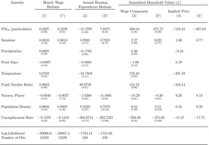
Table 1 presents results for two versions of the model. In the …rst, the wage and housing
expenditure equations are estimated with the full set of amenities described above. The
resulting coe¢cients, and associated t-statistics, are presented in columns 1 and 2.10 The
annualised household wage component is shown in column 3, and this is then combined with
column 2 - as indicated by equation (4) above - to yield the implicit prices in column 4.11 These
prices represent the amount that the average household is willing to pay for the amenity at
the margin (in 1995 prices).
As a group, the amenities are highly statistically signi…cant in both the wage and housing
expenditure equations.12 Individually, …ve of the amenities are statistically signi…cant at the
1% level or better in at least one of the equations. The exceptions are three of the climate
9Only local authority provided and registered day nurseries.
10Findings for individual worker characteristics and housing types are reported in the appendix.
11The housing expenditure component is simply the linearised regression coe¢cient. Linearisation was
carried out as follows: b0=by(1¡¸)whereb0 is the linearised coe¢cient,bthe regression coe¢cient andyis the
sample mean annual housing expenditure or hourly wage. The wage component is the linearised coe¢cient multiplied by the product of average hours per week (38.34), weeks per year (45.63) and workers per household (1.29).
12Likelihood ratio tests indicate that the amenities are jointly signi…cant at above the 1% level in both
Table 1: Regression Results and Hedonic Price Estimates
Amenity Hourly Wage Annual Housing Annualized Household Values($)
Hedonic Expenditure Hedonic
Wage Component Implicit Price
(1) (10) (2) (20) (3) (30) (4) (40)
PM10 (particulates) 0:2207
(5:36) 0(7:2108:61) ¡21(0::33)3767 7(0:8875:20) 498(5:36):04 475(0:20):72 ¡519:42 ¡467:84
Sunshine 0:0010
(1:69) 0(4:0013:18) 3(4:9285:11) 3(6:7925:77) (12::2769) 3(6:021:77) 1:66 0:77
Precipitation 0:0001
(0:59) ¡0(0::178360) (00::2659) ¡0:44
Frost Days ¡0:0007
(0:19) ¡0(0::806515) ¡(01:19):60 0:79
Temperature 0:0782
(0:82) ¡24(0::17)7958 176(0:82):43 ¡201:23
Pupil Teacher Ratio 0:0683
(0:90) 49(0:9759:61) 154(0:90):12 ¡104:14
Nursery Places ¡0:0046
(2:01) ¡0(1::003773) ¡1(0::026828) ¡0(0::190805) ¡(210:01):29 ¡(08:05):38 9:26 8:18
Population Density 0:0002
(3:85) 0(4:0002:30) 0(9:8332:57) 0(10:7879:52) (30::4285) (100:41:52) 0:42 0:38
Unemployment Rate ¡0:1279
(6:20) ¡0(6::121965) ¡304(10::72)0741 ¡292(12::08)7231 ¡288(6:20):60 ¡(12275:08):02 ¡15:47 ¡17:71
Log-Likelihood ¡30066:6 ¡30067:4 ¡1724:14 ¡1724:93
Number of Obs. 12320 12320 220 220
variables - precipitation, temperature and frost days - and the pupil-teacher ratio. The climate
variables exhibit multicollinearity for obvious reasons; in the case of the pupil-teacher ratio, the
lack of signi…cance may indicate that county level data is too coarse to detect an e¤ect on wages
or house prices. The quality of primary and secondary education varies considerably within
each of the counties, and therefore may in‡uence the choice of location within, rather than
between, counties. In the light of these considerations, the model was re-estimated without
precipitation, temperature, frost days and the pupil-teacher ratio. The results, presented in
columns 1’, 2’, 3’and 4’, indicate that the change in speci…cation has little impact on either the
wage and housing expenditure coe¢cients or, more importantly, the implicit prices. Moreover,
as we shall see later, the quality of life ranking is robust to the change. For the remainder of
the paper we focus discussion on the second version of the model.
When interpreting the results, it is important to recall that whilst locational traits that
enhance utility should have a positive price, and undesirable traits a negative price, the
un-derlying wage and housing expenditure coe¢cients may be ambiguous in sign.
The negative price of airborne particles,P M10, conforms with a priori expectations. One
question that arises is whether this result re‡ects not just a distaste for poor air quality, but
also a response to other externalities - such as noise and visual intrusion - associated with
the production of P M10: In the UK, in 1995, the main sources of P M10 emissions were road
transport (26%), power stations (15%) and iron and steel production (9%). Re…neries,
con-struction, mining, quarrying and ‘other industrial processes’ together accounted for a further
37% of the total. Each of these activities is clearly capable of generating a variety of forms
of externality. However, airborne particles are, by nature, highly mobile - especially when
emitted from industrial chimneys. Detection may therefore take place some distance from the
point of emission, thereby limiting the degree to which our measure of air quality is acting as
a proxy for other variables.
We …nd that sunshine makes a positive contribution to the quality of life in England and
Wales as, not surprisingly, does the level of nursery provision. Unemployment, similarly, has
its expected negative price. Population density is di¢cult to sign a priori because, as Rosen
distaste for density as such. Thus its positive price may, in part, re‡ect the fact that regions
which are more densely populated can support a wider range of consumption activities.
These results are in line with existing research. For Britain, Maddison (1997), using
di¤erent data on wages and house prices, similarly found that sunshine and population density
made a positive contribution to the quality of life, whereas unemployment had a negative e¤ect.
Whilst nursery provision was not examined, he did …nd that the proportion of children who
passed …ve or more GCSEs had a positive price.
Our estimates of the impact of airborne particulates on the quality of life are the …rst
for the UK. For the US, Roback (1982), Blomquist, Berger and Hoehn (1988) and Gyourko
and Tracy (1991) all found that particulates had a negative price. In addition, their results
suggest that, as in England and Wales, both sunshine and population density make a positive
contribution to the quality of life.13
The implicit prices in Table 1 are used to construct quality of life (QOL) index values for
each county as follows:
QOLk=
X
Pm¤amk (8)
where Pm¤ is the implicit price of amenity m andamk is the quantity of amenitym in county
k.
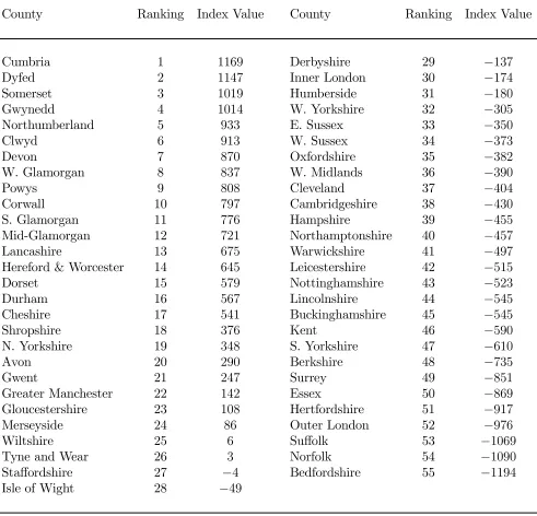
We have standardised on a hypothetical county which has the sample mean quantity of
each amenity. Table 2 presents the standardised quality of life index value for each county, in
descending order. The top-ranked county is Cumbria in the north-west of England, followed
by Dyfed in Wales and then Somerset in the south-west of England. The standardised QOL
index value for Cumbria is £1169, which represents the amount that the average household
would be willing to pay per year to live in Cumbria rather than the hypothetical average
county. At the other end of the scale is Bedfordshire with a value of £-1194, giving an overall
QOL range in England and Wales of £2363 per annum. It is important to bear in mind that
these results do not imply any tendency for migration from low to high-ranked counties. The
model is an equilibrium one in which counties that are ranked highly in terms of QOL have
13All three US studies …nd that hours of sunshine has a positive price. Roback is the only one of the three
to include population density among the regressors.
Table 2: Quality of Life by County
County Ranking Index Value County Ranking Index Value
Cumbria 1 1169 Derbyshire 29 ¡137
Dyfed 2 1147 Inner London 30 ¡174
Somerset 3 1019 Humberside 31 ¡180
Gwynedd 4 1014 W. Yorkshire 32 ¡305
Northumberland 5 933 E. Sussex 33 ¡350
Clwyd 6 913 W. Sussex 34 ¡373
Devon 7 870 Oxfordshire 35 ¡382
W. Glamorgan 8 837 W. Midlands 36 ¡390
Powys 9 808 Cleveland 37 ¡404
Corwall 10 797 Cambridgeshire 38 ¡430
S. Glamorgan 11 776 Hampshire 39 ¡455
Mid-Glamorgan 12 721 Northamptonshire 40 ¡457
Lancashire 13 675 Warwickshire 41 ¡497
Hereford & Worcester 14 645 Leicestershire 42 ¡515
Dorset 15 579 Nottinghamshire 43 ¡523
Durham 16 567 Lincolnshire 44 ¡545
Cheshire 17 541 Buckinghamshire 45 ¡545
Shropshire 18 376 Kent 46 ¡590
N. Yorkshire 19 348 S. Yorkshire 47 ¡610
Avon 20 290 Berkshire 48 ¡735
Gwent 21 247 Surrey 49 ¡851
Greater Manchester 22 142 Essex 50 ¡869
Gloucestershire 23 108 Hertfordshire 51 ¡917
Merseyside 24 86 Outer London 52 ¡976
Wiltshire 25 6 Su¤olk 53 ¡1069
Tyne and Wear 26 3 Norfolk 54 ¡1090
Sta¤ordshire 27 ¡4 Bedfordshire 55 ¡1194
Isle of Wight 28 ¡49
Table 3: Impact of Amenities on Quality of Life
Amenity Value Range (£) Inter-quartile Range (£)
PM10(particulates) 4678.35 935.67
Sunshine 395.69 136.33 Nursery Places 557.32 200.91 Population Density 3173.47 154.69 Unemployment Rate 216.02 59.32
correspondingly higher house prices and/or lower wage rates.
To help understand the ranking, we …rst consider the relative contribution of each amenity
to the QOL index, and then look at the pattern of amenities across counties.
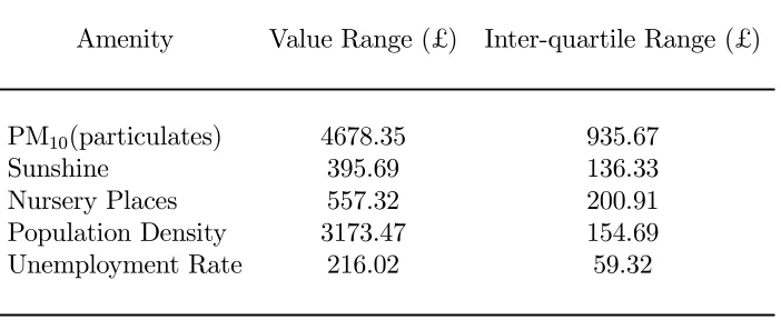
An indication of the contribution of each amenity to the QOL index is the amount that
a household would be willing to pay to move from the county with the lowest amount of a
particular amenity to the county with the highest. This range is presented in column 2 of Table
3, and suggests that the main contributors to the index are the measure of air quality (a range
of £4678) and population density (a range of £3173). The contributions of the remaining three
variables are appreciably smaller; the next largest being nursery provision with a range of £557,
followed by sunshine, £396, and unemployment, £ 216. The ranges for both air quality and
population density are substantially higher than the overall QOL range of £2363, re‡ecting a
tendency for good air quality to be associated with low population density. The inter-quartile
range, in column 3, con…rms the importance of air quality but reveals that towards the centre
of the distribution the relative contribution of population density is diminished.
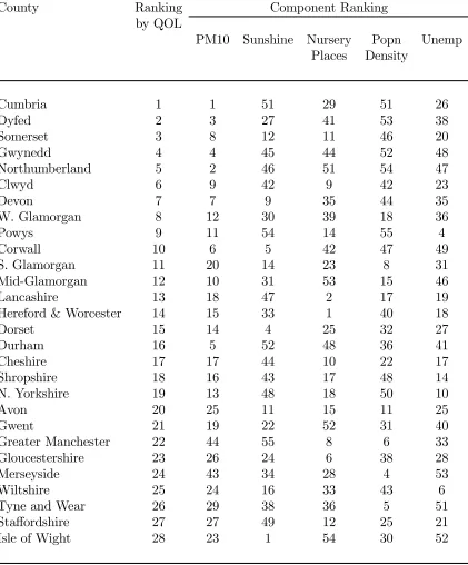
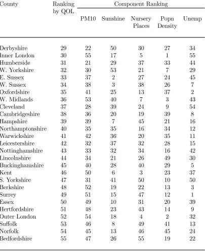
Table 4 presents the overall QOL ranking together with rankings for each of the amenities.
For each amenity, the numbers indicate the preference ranking; thus, for P M10 number 1 is
assigned to the county with the lowest level (because it has a negative price), but for sunshine
(which has a positive price) number 1 indicates the highest number of hours. The most
striking characteristic of the counties at the top of the overall ranking is that they enjoy good
air quality: of the top ten QOL counties, eight are ranked among the ten best for air quality.
They also tend to be characterised by low population densities, with seven of the top ten
overall being among the ten with the lowest densities. In other respects the counties at the
top exhibit considerable variation. For instance, they include the …fth and …fty-fourth ranked
counties in terms of sunshine, the fourth and forty-ninth in terms of unemployment, and the
ninth and …fty-…rst in terms of nursery provision. This heterogeneity is not unexpected given
that these amenities have small value ranges relative to air quality and population density.
The ten counties at the bottom of the QOL ranking are not quite a mirror image of those at
the top. They are characterised by poor air quality, but there is little uniformity in population
density. The group includes Outer London, which has the second highest density, but also
Su¤olk and Norfolk, which have very low densities. In fact, only Outer London and South
Yorkshire from this group feature among the ten counties with the highest population density.
With regard to the other amenities, the picture is mixed. As well as counties that perform
poorly, the group includes Kent, which is third in the list of nursery provision and sixth in the
sunshine ranking, and Surrey, which has the lowest unemployment rate of all regions.
The correlation between air quality and overall QOL, whilst strong, is by no means perfect.
For instance, both Inner London and Greater Manchester achieve a QOL rank more than
twenty places above their respective air quality rankings. In the case of Inner London, the
explanation lies in good nursery provision, plenty of sunshine and, most importantly, a high
population density. The density in Inner London, just over eight thousand three hundred
people per square kilometre, is more than twice the …gure in the next most densely populated
region. Greater Manchester also bene…ts from good nursery provision and a high density
(almost twice as high as the next county in the density ranking) - which more than compensate
for having the least amount of sunshine of all counties. South Yorkshire, by contrast, has a
QOL rank sixteen places below its air quality position. This is due to a combination of low
sunshine, high unemployment and poor nursery provision.
As a check on the robustness of the results, we computed an alternative QOL ranking
based upon the implicit prices reported in column 4 of Table 1. The two rankings are broadly
consistent, with a Spearman rank correlation coe¢cient of 0.98. This is evident both at the
Table 4: Overall Quality of Life and Component Rankings
County Ranking Component Ranking by QOL
PM10 Sunshine Nursery Popn Unemp Places Density
Cumbria 1 1 51 29 51 26
Dyfed 2 3 27 41 53 38
Somerset 3 8 12 11 46 20
Gwynedd 4 4 45 44 52 48
Northumberland 5 2 46 51 54 47
Clwyd 6 9 42 9 42 23
Devon 7 7 9 35 44 35
W. Glamorgan 8 12 30 39 18 36
Powys 9 11 54 14 55 4
Corwall 10 6 5 42 47 49
S. Glamorgan 11 20 14 23 8 31 Mid-Glamorgan 12 10 31 53 15 46 Lancashire 13 18 47 2 17 19 Hereford & Worcester 14 15 33 1 40 18
Dorset 15 14 4 25 32 27
Durham 16 5 52 48 36 41
Cheshire 17 17 44 10 22 17
Shropshire 18 16 43 17 48 14 N. Yorkshire 19 13 48 18 50 10
Avon 20 25 11 15 11 25
Gwent 21 19 22 52 31 40
Greater Manchester 22 44 55 8 6 33 Gloucestershire 23 26 24 6 38 28 Merseyside 24 43 34 28 4 53
Wiltshire 25 24 16 33 43 6
Tyne and Wear 26 29 38 36 5 51 Sta¤ordshire 27 27 49 12 25 21 Isle of Wight 28 23 1 54 30 52
Table 4: continued
County Ranking Component Ranking by QOL
PM10 Sunshine Nursery Popn Unemp Places Density
Derbyshire 29 22 50 30 27 34 Inner London 30 55 17 5 1 55 Humberside 31 21 29 37 33 44 W. Yorkshire 32 30 53 21 7 29 E. Sussex 33 37 2 27 24 45
W. Sussex 34 38 3 38 26 7
Oxfordshire 35 41 25 13 37 2 W. Midlands 36 53 40 7 3 43 Cleveland 37 28 39 24 9 54 Cambridgeshire 38 36 20 19 39 8 Hampshire 39 39 7 45 21 16 Northamptonshire 40 35 35 16 34 12 Warwickshire 41 42 36 20 35 11 Leicestershire 42 32 37 32 28 15 Nottinghamshire 43 33 32 34 16 42 Lincolnshire 44 34 21 26 49 30 Buckinghamshire 45 40 28 40 29 5
Kent 46 50 6 3 23 37
S. Yorkshire 47 31 41 50 10 50 Berkshire 48 52 19 22 13 3
Surrey 49 51 15 47 12 1
Essex 50 49 10 31 20 39
Hertfordshire 51 48 23 43 14 9 Outer London 52 54 18 4 2 32
Su¤olk 53 46 8 49 41 13
Norfolk 54 45 13 46 45 24
is same ten counties that have the lowest QOL indices.
Notwithstanding this robustness with regard to speci…cation, the QOL ranking must be
treated with caution. First, the housing data permitted only a limited degree of control
for quality di¤erences. This contrasts with the highly detailed information on individuals’
personal and job characteristics. Second, there may be important regional variations that
are not captured by our set of amenities. QOL indices based on a di¤erent set of locational
traits could potentially generate a substantially di¤erent ranking. Third, the implicit prices are
based on an assumption regarding the “marginal” household - the household that is indi¤erent
between locations. In common with previous work, we have taken this to be the household
with the sample mean values of hours per worker and workers per household. Finally, the
implicit prices are de…ned for small changes in locational attributes and therefore estimates
of willingness to pay for substantial improvements in amenity levels are approximations.
4 Conclusions
In this paper we have applied an extended version of Roback’s (1982) general equilibrium
lo-cation model to individual and county level data from England and Wales to estimate implicit
prices for a variety of locational attributes. We found positive prices for population density,
nursery provision and hours of sunshine, and negative prices for air pollution and
unemploy-ment. The implicit prices were used to compute an overall Quality of Life index value for each
of the counties. For the representative household, the di¤erence in Quality of Life between the
top-ranked and bottom-ranked county was estimated at £2363 per year. The highest ranked
counties are characterised by low levels of airborne particulates and population density, but
are heterogeneous in other respects. Those at the bottom of the ranking exhibited even more
variety, having only high levels of airborne particulates in common.
We have emphasised that the implicit prices and associated Quality of Life index values
should be treated with caution but, being derived from the actual decisions of agents, they may
constitute a useful counterpoint to quality of life assessments based on subjective valuations.
Appendix
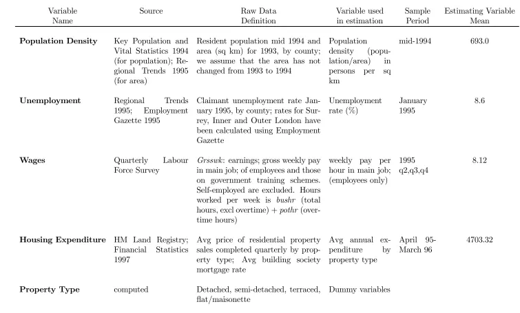
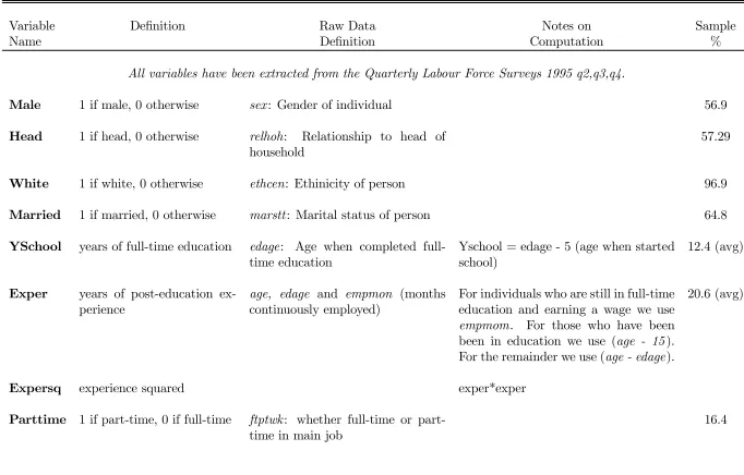
The source and description of each variable used in the estimations is given in Table 5. Table 6
gives a description of the variables representing personal characteristics of individuals. These
variables were included in the wage equation. Table 7 provides the Box-Cox FIML coe¢cients
estimates for all the variables used in the estimations.
Likelihood Ratio Test
To test if the amenities were jointly signi…cant in each equation a likelihood ratio test
was carried out. In the wage equation, the restricted model was one which only contained
the constant and personal characteristics as explanatory variables. In the housing equation,
the restricted model was one which contained the constant and the property dummies as
explanatory variables. The null hypothesis of the coe¢cients on the amenities being jointly
equal to zero was tested against the alternative that at least one of the amenity coe¢cients
was not equal to zero.
The likelihood value from the restricted model was calculated in two ways. (a) The
Box-Cox value for ¸ (see Equation (7)) in the restricted model was kept at that which maximised
the likelihood value of the unrestricted model. (b) The Box-Cox value for ¸ restricted model
was kept at that which maximised the likelihood value of the restricted model.
Thus two likelihood ratio tests were conducted for each equation as represented by Columns
(1),(10), (2) and (20) in Table 1. Using critical values ofÂ2;0:01
9 = 21:66 and 2;0:01
5 = 15:09the
null hypothesis was rejected in the direction of the alternative for all equations.
Acknowledgements
P M10 data has been made available by the Department of the Environment, Transport
and the Regions and AEA Technology, National Environmental Technology Centre.
The climate data has been supplied by the Climatic Research Unit, University of East
An-glia (Climate Impacts LINK Project, Department of the Environment Contract EPG 1/1/16)
on behalf of the Hadley Centre and the Meteorological O¢ce.
Material from the Quarterly Labour Force Surveys is Crown copyright; has been made
permission. Neither the ONS nor The Data Archive bear any responsibility for the analysis
or interpretation of the data reported here.
Table 5: Data Description: Main Variables
Variable Source Raw Data Variable used Sample Estimating Variable
Name De…nition in estimation Period Mean
PM10 (particulates) AEA Technology ¹gm¡3, annual means, grid data
(1km) ¹gm
¡3, annual
mean, by county 1994 17.22
Sunshine Climatic Research
Unit, UEA Sunshine hours (hours x 10) av-eraged over 1961-1990, by month; grid data (mean altitude values) (10 km)
Annual sunshine
hours, by county Average1961-1990 1429
Precipitation Climatic Research
Unit, UEA
Preciptation (mm x 10) averaged over 1961-1990, by month; grid data (mean altitude values) (10 km)
Annual precipita-tion (mm), by county
Average 1961-1990
872.78
Frost Days Climatic Research
Unit, UEA
Frost days (days x 10) averaged over 1961-1990, by month; grid data (mean altitude values) (10 km)
Annual frost days, by county
Average 1961-1990
103
Temperature Climatic Research
Unit, UEA
Degrees centigrade averaged over 1961-1990, by month; grid data (mean altitude values) (10 km)
Annual average temperature, by county Average 1961-1990 8
Pupil-Teacher Ratio Regional Trends 1996 Primary and Secondary school ra-tios, by county
Average Pupil-Teacher ratio
1994/95 19.7
Nursery Places Regional Trends 1996 Day nursery places per 1000 popu-lation aged under 5 years, by county
Nursery Places March 1994
Table 5: continued
Variable Source Raw Data Variable used Sample Estimating Variable
Name De…nition in estimation Period Mean
Population Density Key Population and Vital Statistics 1994 (for population); Re-gional Trends 1995 (for area)
Resident population mid 1994 and area (sq km) for 1993, by county; we assume that the area has not changed from 1993 to 1994
Population
density (popu-lation/area) in persons per sq km
mid-1994 693.0
Unemployment Regional Trends
1995; Employment Gazette 1995
Claimant unemployment rate Jan-uary 1995, by county; rates for Sur-rey, Inner and Outer London have been calculated using Employment Gazette Unemployment rate (%) January 1995 8.6
Wages Quarterly Labour
Force Survey
Grsswk: earnings; gross weekly pay in main job; of employees and those on government training schemes. Self-employed are excluded. Hours worked per week is bushr (total hours, excl overtime) +pothr (over-time hours)
weekly pay per hour in main job; (employees only)
1995 q2,q3,q4
8.12
Housing Expenditure HM Land Registry; Financial Statistics 1997
Avg price of residential property sales completed quarterly by prop-erty type; Avg building society mortgage rate
Avg annual ex-penditure by property type
April
95-March 96 4703.32
Property Type computed Detached, semi-detached, terraced,
‡at/maisonette
Dummy variables
Table 6: Data Description: Personal Characteristics in Wage Equation
Variable De…nition Raw Data Notes on Sample
Name De…nition Computation %
All variables have been extracted from the Quarterly Labour Force Surveys 1995 q2,q3,q4.
Male 1 if male, 0 otherwise sex: Gender of individual 56.9
Head 1 if head, 0 otherwise relhoh: Relationship to head of
household 57.29
White 1 if white, 0 otherwise ethcen: Ethinicity of person 96.9
Married 1 if married, 0 otherwise marstt: Marital status of person 64.8
YSchool years of full-time education edage: Age when completed full-time education
Yschool = edage - 5 (age when started school)
12.4 (avg)
Exper years of post-education ex-perience
age, edage and empmon (months
continuously employed)
For individuals who are still in full-time education and earning a wage we use
empmom. For those who have been been in education we use (age - 15). For the remainder we use (age - edage).
20.6 (avg)
Expersq experience squared exper*exper
Parttime 1 if part-time, 0 if full-time ftptwk: whether full-time or
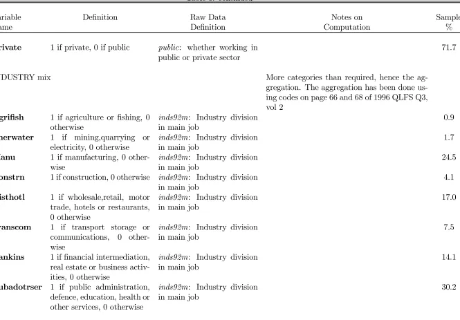
Table 6: continued
Variable De…nition Raw Data Notes on Sample
Name De…nition Computation %
Private 1 if private, 0 if public public: whether working in public or private sector
71.7
INDUSTRY mix More categories than required, hence the ag-gregation. The aggregation has been done us-ing codes on page 66 and 68 of 1996 QLFS Q3, vol 2
Agri…sh 1 if agriculture or …shing, 0 otherwise
inds92m: Industry division in main job
0.9
Enerwater 1 if mining,quarrying or electricity, 0 otherwise
inds92m: Industry division in main job
1.7
Manu 1 if manufacturing, 0
other-wise inds92min main job: Industry division 24.5
Constrn 1 if construction, 0 otherwise inds92m: Industry division in main job
4.1
Disthotl 1 if wholesale,retail, motor trade, hotels or restaurants, 0 otherwise
inds92m: Industry division in main job
17.0
Transcom 1 if transport storage or communications, 0 other-wise
inds92m: Industry division in main job
7.5
Bankins 1 if …nancial intermediation, real estate or business activ-ities, 0 otherwise
inds92m: Industry division in main job
14.1
Pubadotrser 1 if public administration, defence, education, health or other services, 0 otherwise
inds92m: Industry division in main job
30.2
Table 6: continued
Variable De…nition Raw Data Notes on Sample
Name De…nition Computation %
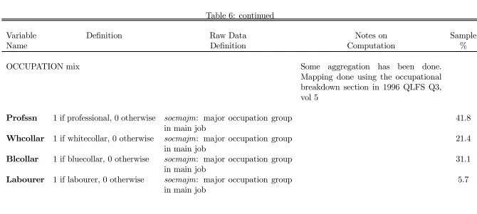
OCCUPATION mix Some aggregation has been done. Mapping done using the occupational breakdown section in 1996 QLFS Q3, vol 5
Profssn 1 if professional, 0 otherwise socmajm: major occupation group
in main job 41.8
Whcollar 1 if whitecollar, 0 otherwise socmajm: major occupation group in main job
21.4
Blcollar 1 if bluecollar, 0 otherwise socmajm: major occupation group in main job
31.1
Labourer 1 if labourer, 0 otherwise socmajm: major occupation group
Table 7: FIML estimates of Wage and Housing Equation
Wage Equation Housing Equation
Variable Estimate t-statistic Estimate t-statistic
Constant -0.63370 6.10 3.85905 119.01 Male 0.154066 10.97
Head 0.14783 10.62 White 0.24930 9.32 Married 0.09240 8.52 YSchool 0.07090 34.20 Exper 0.04195 26.78 Expersq -0.00074 24.17 Parttime -0.15320 10.80 Private -0.18638 13.25 Agri…sh -0.19915 4.02 Enerwater 0.32538 7.82 Manu 0.15064 9.03 Constrn 0.09858 3.58 Disthotl -0.09192 5.31 Transcom 0.07850 4.01 Bankins 0.20700 12.60 Profssn 0.61837 26.02 Whcollar 0.24655 10.02 Blcollar 0.16102 6.79
Detached 0.15816 31.47
Semidetached 0.05851 10.56
Terraced 0.01036 2.13
PM10(particulates) .03200 7.60 0.00031 0.20
Sunshine .00020 4.18 0.00015 6.77 Nursery Places -.00056 1.73 -0.00001 -0.05 Population Density .00003 4.30 0.00003 10.52 Unemployment Rate -.01850 6.65 -0.01147 -12.08
No of Observations 12320 220 Log likelihood -30067.40 -1724.93
In the wage equation, the omitted industry is “public administration and other services” and the omitted occupation is “labourer”.
In the housing equation, the omitted property type is “‡at/maisonette”.
References
Blomquist, G.C., Berger, M.C. and Hoehn, J.P. (1988). ‘New Estimates of the Quality
of Life in Urban Areas.’ American Economic Review, vol. 78, pp. 89-107.
Clarke, D.E. and Nieves, L.A. (1994). ‘An Interregional Hedonic Analysis of Noxious
Facility Impacts on Local Wages and Property Values.’ Journal of Environmental Eco-nomics and Management, vol. 27, pp. 235-53.
Department of the Environment, Transport and the Regions (1999). A Better Quality of Life: A Strategy for Sustainable Development in the United Kingdom. TSO, London. Command number 4345.
Gyourko, J. and Tracy, T. (1991). ‘The Structure of Local Public Finance and the
Quality of Life.’ Journal of Political Economy, vol. 99, pp. 774-806.
Maddison, D. (1997). ‘Measuring the Impact of Climate Change on Britain.’
unpub-lished PhD thesis, University of Strathclyde.
Nordhaus, W. and Tobin, J. (1972). ‘Is Growth Obsolete?’ In Economic Growth. New York: National Bureau of Economic Research.
Ridker, G. and Henning, J.A. (1967). ‘The Determinants of Residential Property Values
with Special Reference to Air Pollution.’ Review of Economics and Statistics, vol. 49, pp. 246-57.
Roback, J. (1982). ‘Wages, Rents, and the Quality of Life.’ Journal of Political Economy, vol. 90, pp. 1257-1278.
Rosen, S. (1974). ‘Hedonic Prices and Implicit Markets: Product Di¤erentiation in Pure
Competition.’Journal of Political Economy, vol. 82, pp. 34-55.
Stedman, J. Campbell, G and Vincent, K. (1997). ‘Estimated High Resolution Maps of
Background Air Pollutant Concentrations in the UK.’ AEA/RAMP/20008001/003.