Privacy Preserving Fuzzy Modeling for Secure Multiparty Computation

Privacy Preserving Fuzzy Modeling for Secure

Multiparty Computation

Hirofumi Miyajima

†1

, Noritaka Shigei

†2

, Hiromi Miyajima

†3

, Yohtaro Miyanishi

†4

Shinji Kitagami

†5

and Norio Shiratori

†6

Abstract—Many studies on privacy preserving of machine learning and data mining have been done in various methods by use of randomization techniques, cryptographic algorithms, anonymization methods, etc. Data encryption is one of typical approaches. However, its system requires both encryption and decryption for requests of client or user, so its complexity of computation is very high. Therefore, studies on secure computation using shared data are made to avoid secure risks being abused or leaked and to reduce computing cost. The secure multiparty computation (SMC) is one of these methods. So far, some studies have been done with SMC, but complex calculation processing such as machine learning has never proposed yet. In the previous paper, we proposed BP learning method for SMC on cloud computing system. In this paper, we propose learning method(Fuzzy modeling) of fuzzy inference system for SMC and prove the validity of it. Further, the performance of the proposed method is shown in numerical simulations.

Index Terms—cloud computing, secure multiparty computa-tion, fuzzy modeling, control problem.

I. INTRODUCTION

P

RIVACY preserving machine learning and data mining can be achieved in various methods by use of random-ization techniques, cryptographic algorithms, anonymrandom-ization methods, etc [1]–[6]. However, data encryption system re-quires both encryption and decryption for requests of client or user, so its complexity is very high. The problem is the trade-off between the security and the complexity. As one of these studies, secure multiparty computation (SMC) has been introduced [7]–[9]. The purpose of SMC is to allow servers(parties) to carry out distributed computing tasks in secure way. As one of them, SMC systems sharing data itself to each party attract attention, and some studies with them have been done. A simple method to share data was proposed and they were applied to some problems [10], [11]. In the previous paper, we proposed BP learning for neural networks and clustering methods for SMC [12], [13]. In this paper, we propose learning method(fuzzy modeling) of fuzzy inference systems for SMC and show the effectiveness of them in numerical simulations. The difference between BP learning

Affiliation: Graduate School of Science and Engineering, Kagoshima University, 1-21-40 Korimoto, Kagoshima 890-0065, Japan

corresponding auther to provide email: [email protected]

†1email: [email protected] †2email: [email protected] †3email: [email protected]

Affiliation: Information Systems Engineering and Management, Tokyo, Japan

†4email: [email protected]

Affiliation: Waseda University Graduate School of Global Information and Telecommunication Studies(GITS), Tokyo, Japan

†5email: [email protected]

Affiliation: Waseda University GITS, Tokyo, Japan

[image:1.595.348.506.193.328.2]

†6email: [email protected]

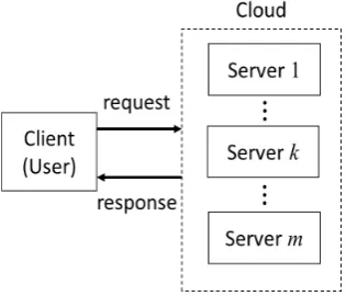
Fig. 1. A configuration of cloud computing system.

and fuzzy modeling is as follows [14] : In BP learning input and output relation for learning data is represented as weights of neurons of neural network, but it is difficult to know the interpretability of input and output learning data. In fuzzy modeling, input and output relation for learning data is represented as fuzzy rules for fuzzy inference system and it is easy to understand the interpretability of input and output learning data. In this paper, we will show this relation using a control problem. In Section 2, we describe the idea for sharing data securely. Further, we also introduce the conventional learning algorithm for fuzzy inference systems. In Section 3, we describe our proposed learning algorithm for SMC. In Section 4, some simulation results are presented to demonstrate the effectiveness of the proposed method.

II. PRELIMINARY

A. System configuration of cloud system and related works

Fig.1 shows a system for SMC of cloud computing. The system is composed of a client and cloud with m

servers(parties) [12]. The client sends data to each server and each server memorizes them. If the client requires data processing, each server performs one’s computation and sends each result to client. The client computes the final result using them. If the result is not obtained by one processing, data processing between client and servers are iterated until the final result is obtained. The problem is how data are shared and the computation for each server is carried out.

First, let us explain about horizontally partitioned method(HPM) using Table 1. All the dataset are divided into two servers, Server 1 and 2 as follows:

Server 1: dataset for ID=1, 2 Server 2: dataset for ID=3, 4.

In this case, two averages with subsets A and B for Server 1 are computed as(90 + 60)/2and(55 + 82)/2, respectively. Likewise, two averages with subsets A and B for Server 2 are (70 + 40)/2 and(30 + 70)/2, respectively. As a result, two averages for subsets A and B are 65.0 and 59.25, respectively. These are obtained as the sums of average ofa(1) _anda(2)_,

and of b(1) _{and b}(2)_{,where a =a}(1)_+a(2) _{andb =b}(1)₊ b(2). Each server cannot know half of the dataset, so privacy preserving holds.

Likewise, vertically partitioned method(VPM) is intro-duced. In this care, dataset for subject A and B are assigned to Server 1 and 2, respectively.

At third, let us consider about any partitioned method for SMC. All the dataset are divided into two parties, mixed horizontally and vertically partitioned data. These methods need a large number of learning data to keep security, but the proposed method using secure shared data seems to keep them by small number of data.

B. The representation of secure shared data

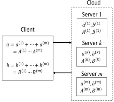
Let us explain data representation for the proposed method using Fig.2 [10], [11]. Let a and b be two positive integers. First, two integers aandb are shared into m real numbers. Let a=a(1)+· · ·+a(m) andb=b(1)+· · ·+b(m) as the addition form and a =A(1)_{· · ·A}(m) _{and b =B}(1)_{· · ·B}(m)

as the multiplication form. Then the following results hold: 1)a+b= (a(1)_+b(1)_{) +· · ·+ (a}(m)_+b(m)₎

2)a−b= (a(1)_−b(1)_{) +· · ·+ (a}(m)_−b(m)₎

3)ab= (A(1)B(1))· · ·(A(m)B(m)) 4)a/b= (A(1)/B(1))· · ·(A(m)/B(m))

That is, four basic operations of arithmetic (addition, sub-traction, multiplication, and division) hold as integration of the result computed independently by each server [11], [12]. In this paper, a(k) _andA(k) _{for 1≤k < m−1 are selected}

randomly in [0,1] and [−1,1], respectively. Further, a(m)

andA(m) _{are selected asa−}∑m−1

k=1 a

(k)_anda/Πm−1

k=1A (k)_,

respectively.

Let us show an example of shared data using Table I as follows [11]:

a=a(1)_+a(2) _:a(1)_=a(r

1/10)anda(2) =a(1−r1/10), b=b(1)_+b(2) _:b(1)_=b(r

1/10)andb(2)=b(1−r2/10), a=A(1)_A(2) _:A(1)₌√_a(r

1/10)andA(2)=

√

a(10/r1), b=B(1)B(2) : B(1) =√b(r2/10) andB(2) =

√

b(10/r2)

, where r1 and r2 are real random numbers for −9≤r1≤9

and0.2≤r2≤9,r1̸=1,r2̸=1, respectively. For example,a(1)

anda(2) _{for ID=1 are computed asa}(1)_{= 90×(2/10) = 18}

and a(2) _{= 90×(1−2/10) = 72 and data A}(1) _{and A}(2)

for ID=1 are computed asA(1)₌√_{90×(4/10) = 3.79and} A(2) =√90×(10/4) = 23.71, respectively. Note that Server 1 has all the data in column-wise ofa(1),b(1),A(1)andB(1)

for each ID and Server 2 has all the data in column-wise of

[image:2.595.331.521.61.232.2]

a(2),b(2),A(2) andB(2) for each ID as shown in Table.I. Remark that each data for server is randomized and the method does not need to use encrypted data.

Fig. 2. The representation of secure shared data.

C. The conventional fuzzy inference system

The conventional fuzzy inference system is described [14]. LetZj={1,· · ·, j} for the positive integerj. LetR be the set of real numbers. Let x= (x1,· · ·, xN)andy∗ be input and output data, respectively, wherexj∈R for j ∈ZN and

y∗∈R. Then the rule of fuzzy inference model is expressed as

Ri : if x1 isMi1 and · · · andxN is MiN

theny is ci (1)

, where i ∈ Zn is a rule number, j ∈ ZN is a variable number, Mij is a membership function of the antecedent part, andci is a real number of the consequent part.

A membership value of the antecedent part µj for input

xis expressed as

µi= N

∏

j=1

Mij(xj). (2)

If Gaussian membership function is used, then Mij is expressed as follow

Mij = exp

(

−1

2

(

xj−aij

bij

)2)

. (3)

, where aij andbij are the center and the width values of

Mij, respectively.

The output y∗ of fuzzy inference is calculated by the following equation:

y=

∑n

i=1µi·ci

∑n i=1µi

. (4)

D. Learning algorithm for the conventional model

In order to construct the effective model, the conven-tional learning method is introduced. The objective function

E is defined to evaluate the inference error between the desirable output yr _{and the inference output y}∗_{. In this} section, we describe the conventional learning algorithm. Let D={(xp₁,· · ·, xp_N, yr

p)|p∈ZP}be the set of learning data. The objective of learning is to minimize the following mean square error(MSE):

E= 1

P

P

∑

p=1

(yp∗−y r p)

2

TABLE I

DATA ONSERVER1ANDSERVER2.

Additional form Multiplication form

ID subject A subject B a b A B

a b r1 a(1) a(2) b(1) b(2) r2 A(1) A(2) B(1) B(2)

1 90 55 2 18 72 11 44 4 3.79 23.71 2.97 18.54

2 60 82 -3 -18 78 -24.6 106.6 5 3.87 15.49 4.53 18.11

3 70 30 5 35 35 15 15 0.4 0.33 209.17 0.22 136.93

4 40 70 -6 -24 64 -42 112 3 1.90 21.08 2.51 27.89

average 65 59.25 2.75 62.25 -10.15 69.4

, where y_p∗ is the inference output for the p-th inputxp_{. In} order to minimize the objective functionE, each parameter

α∈ {aij, bij, ci}is updated based on the descent method as follows [14]:

α(t+ 1) =α(t)−Kα

∂E

∂α (6)

where t is iteration time and Kα is a constant. When Gaussian membership function fori∈Znandj∈Zmare used, the following relation holds [14].

∂E ∂aij

= ∑nµj i=1µi

·(y−y∗)·(ci−y)·

xj−aij

b2

ij

(7)

∂E ∂bij

= ∑nµi i=1µi

·(y−y∗)·(ci−y)·

(xj−aij)2

b3

ij (8)

∂E ∂ci

= ∑nµi i=1µi

·(y−y∗) (9)

Then, the conventional learning algorithm is shown as follows [14]:

Learning Algorithm A

Step A1 : The threshold θ of inference error and the maximum number of learning time Tmax are given. The initial assignment of fuzzy rules is set to equally intervals. Let nbe the number of rules andn=dmfor an integerd. Lett= 1.

Step A2 : The parametersaij,bijandciare set to the initial values.

Step A3 : Letp= 1.

Step A4 : A data(xp₁,· · ·, xp

m, ypr)∈D is given.

Step A5 : From Eqs.(2) and (4), µi andy∗ are computed.

Step A6 : Parametersaij,bij andciare updated by Eqs.(7), (8) and (9).

Step A7: Ifp=P then go to Step A8 and ifp < P then go to Step A4 withp←p+ 1.

Step A8: Let E(t) be inference error at step t calculated by Eq.(5). If E(t) > θ andt < Tmax then go to Step A3 witht←t+ 1else ifE(t)≤θandt≤Tmaxthen the algorithm terminates.

Step A9: If t > Tmax andE(t)> θ then go to Step A2 withn=dm_{as d←d+ 1andt= 1.}

III. SECURE MULTIPARTY COMPUTATION

Let us consider a system composed of client and m

servers(See Fig.1). In learning on cloud system, learning data and parameters are shared to each server in additional or multiplication forms. Each server updates shared parameters and sends the computation result to the client. The client can get new parameters by additional or multiplying the results of m servers. The process is iterated until the error (difference)

between the output of the system and the desired output becomes sufficiently small. The problem is how parameters on the user are updated using the set of learning data shared on each server. The shared representation of learning data

{(xl_{, d(x}l_))|l∈Z

P}and parameters are given as follows:

xl=(xl1,· · ·, xlj,· · ·, xlN

)

(10)

forl∈ZP and

xl_j=

m

∑

k=1

(xl_j)k (11)

fori∈ZN,

d(xl) =

m

∑

k=1

(d(xl))k (12)

, whered(xl_{) is the desirable output for the input x}l_{. Note} that Eqs.(11) and (12) are in additional form for shared data. In this case, Eqs.(7), (8) and (9) are renewed as follows:

△akij =

µj

∑n i=1µi

·(y−y∗)·(ci−y)·

xj−aij

b2

ij (13)

(ak_ij)(t+ 1) = (ak_ij)(t) +K△ak_ij(t) (14)

△bk_ij = ∑nµi i=1µi

·(y−y∗)·(ci−y)

·(xj−aij)2

b3

ij

/bk_ij (15)

(bk_ij)(t+ 1) = (bk_ij)(t) +K△bk_ij(t) (16)

△cki =

µi

∑n i=1µi

·(y−y∗) (17)

(ck_i)(t+ 1) = (ck_i)(t) +K△ck_i(t) (18)

where each of parameters{aij, bij, ci|i∈Zn, j∈ZN} is rep-resented as aij =

∑m k=1a

k

ij, bij = Πmk=1bkij and ci =

∑m k=1c

k

i, respectively.

Eq. (16) means that each server can update the parameter by dividing bybk

ij for the conventional method.

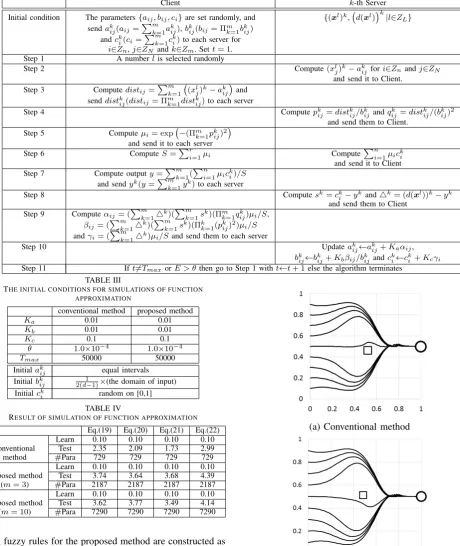
From these results, learning of the fizzy inference system is shown in TableII. The validity of the algorithm is proved from Eqs.(13) to (18). Let us explain the relation between Algorithm A and Table.II.

server. In Step10, aij, bij, and ci are updated. In Step 11, if the error E is sufficient small, or the maximum learning time is attained then the algorithm terminates else go to Step 1.

IV. NUMERICALSIMULATIONS

In this section, numerical simulations of function approx-imation and control problem for conventional and proposed methods are performed. The conventional method means the method without sharing data and the proposed method is ones with m= 3andm= 10.

A. Function Approximation

This simulation uses four systems specified by the fol-lowing functions with 4-dimensional input space [0,1]4(for Eqs.(19) and (20)) and[−1,1]4 (for Eqs.(21) and (22)). The simulation condition is shown in Table III. The numbers of learning and test data selected randomly are 512 and6400, respectively.

y = (2x1+ 4x

2 2+ 0.1)2

37.21 ×

(4 sin(πx3) + 2 cos(πx4) + 6

12

(19)

y = sin(2πx1)×cos(x2)×sin(πx3)×x4+ 1.0 2.0

(20)

y = (2x1+ 4x

2 2+ 0.1)2

74.42 +

4 sin(πx3) + 2 cos(πx4) + 6

446.52

(21)

y = (2x1+ 4x

2 2+ 0.1)2

74.42 +

(3e3x3_{+ 2e}−4x4₎−0.5−_0.077 4.68

(22)

Table IV shows the results of comparison between the conventional and the proposed methods. In each box of Table IV, three numbers from the top to the bottom show MSE of learning (×10−4_{), MSE of test (×10}−4_{) and the number}

of parameters, respectively. The result of simulation is the average value from twenty trials.

The result shows that the accuracy of the conventional and the proposed method is almost the same. Further, it is shown that the results form= 3andm= 10is also about the same accuracy.

B. Obstacle avoidance and arriving at designated point

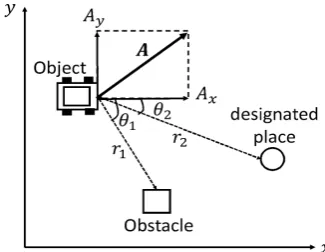
In order to show the interpretability of the proposed model, let us perform simulation of control problem. The problem is how the object avoids the obstacle and arrives at the designated place. As shown in Fig.3, the distance r1 and

the angleθ1between object and obstacle and the distancer2

and the angleθ2between object and the designated place are

selected as input variables, whereθ1 andθ2 are normalized.

Fuzzy inference rules for conventional and proposed method are constructed from learning data ofP= 400points shown in Fig. 4. An obstacle is placed at (0.5,0.5) and a designated place is placed at(1.0,0.5). The number of rules for each method is 81 and the number of attributes is 3. The object moves with the vector A at each step, where Ax of

[image:4.595.340.503.55.181.2]

A is constant andAy of A is output variable. Learning for

Fig. 3. Simulation on obstacle avoidance and arriving at the designated place, whereAxis constant andAyis adjusted.

Fig. 4. Learning data to avoid obstacle and arrive at the designated place (1.0, 0.5).

two methods is successful and the following scenarios are performed.

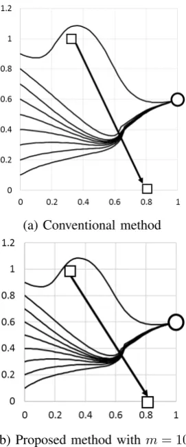
(1)Scenario 1 is simulation for obstacle avoidance and arriving at the designated place when the mobile ob-ject stars from various places (See Fig.5). Fig.5 shows the results of moves of object for starting places at (0.1,0),(0.2,0),· · ·,(0.8,0),(0.9,0) after learning. Simula-tions are successful for all cases. Fig.5 shows the result of conventional and proposed methods form= 10.

(2)Scenario 2 is simulation for the case where the mobile object avoids obstacle placed at different place and arrives at the different designated place. Simulations with obstacle placed at the place (0.4,0.4) and arriving at the designated place (1,0.6) are performed for all cases. The results are successful as shown. Fig.6 shows the result of conventional and proposed methods form= 10.

(3)Scenario 3 is simulation for the case where obstacle moves with the fixed speed. Simulations with obstacle mov-ing with the speed (0.01,0.02) from the place (0.3,1.0) to the place (0.8,0.0) and object arriving at the place (1,0.6) are performed. Simulations are successful for all cases. Fig.7 shows the results of simulations for conventional and proposed methods for m = 10. Since the object does not collide in the obstacle att= 30, thereafter it does not collide in the obstacle.

Lastly, let us consider interpretability of fuzzy rules ob-tained for the proposed method. Let us consider fuzzy rules constructed for the proposed method ofm= 10by learning. Assume that three attributes are short, middle and long for

r1 andr2, minus, central and plus for θ1 and θ2 and left,

[image:5.595.66.527.75.622.2]

TABLE II

LEARNING PROCESS OFFUZZYINFERENCELEARNING FORSMC.

Client k-th Server

Initial condition The parameters{aij, bij, ci}are set randomly, and {(xl)k,

(

d(xl₎)k_|l∈Z L}

sendak ij(aij=

∑m k=1a

k

ij),bkij(bij= Πmk=1bkij)

andck i(ci=

∑m k=1c

k

i)to each server for

i∈Zn,j∈ZNandk∈Zm. Sett= 1.

Step 1 A numberlis selected randomly

Step 2 Compute(xl

j)k−akijfori∈Znandj∈ZN

and send it to Client. Step 3 Computedistij=

∑m k=1

(

(xl j)k−akij

)

and senddistk

ij(distij= Πm_k=1distkij)to each server

Step 4 Computepk

ij=distkij/bkijandqijk =distkij/(bkij)2

and send them to Client.

Step 5 Computeµi= exp

(

−(Πm k=1pkij)2

)

and send it to each server

Step 6 ComputeS=∑r_i=1µi Compute

∑n i=1µic

k i

and send it to Client Step 7 Compute outputy=∑m_k=1(∑n_i=1µick_i)/S

and sendyk_(y=∑m k=1y

k_{)to each server}

Step 8 Computesk_=ck

i−ykand△k= (d(xl))k−yk

and send them to Client Step 9 Computeαij= (

∑m k=1△

k₎₍∑m k=1s

k_)(Πm k=1q

k ij)µi/S,

βij= (

∑m k=1△

k₎₍∑m k=1s

k_)(Πk

k=1(pkij)2)µi/S

andγi= (

∑m k=1△

k_)µ

i/Sand send them to each server

Step 10 Updateak

ij←akij+Kaαij,

bk

ij←bkij+Kbβij/bkijandcki←cki +Kcγi

Step 11 Ift̸=TmaxorE > θthen go to Step 1 witht←t+ 1else the algorithm terminates

TABLE III

THE INITIAL CONDITIONS FOR SIMULATIONS OF FUNCTION APPROXIMATION

conventional method proposed method

Ka 0.01 0.01

Kb 0.01 0.01

Kc 0.1 0.1

θ 1.0×10−4 _1.0×10−4

Tmax 50000 50000

Initialak

ij equal intervals

Initialbk ij

1

2(d−1)×(the domain of input)

Initialck

i random on [0,1]

TABLE IV

RESULT OF SIMULATION OF FUNCTION APPROXIMATION

Eq.(19) Eq.(20) Eq.(21) Eq.(22)

Learn 0.10 0.10 0.10 0.10

conventional Test 2.35 2.09 1.73 2.99

method #Para 729 729 729 729

Learn 0.10 0.10 0.10 0.10

proposed method Test 3.74 3.64 3.68 4.39

(m= 3) #Para 2187 2187 2187 2187

Learn 0.10 0.10 0.10 0.10

proposed method Test 3.62 3.77 3.49 4.14 (m= 10) #Para 7290 7290 7290 7290

main fuzzy rules for the proposed method are constructed as shown in Table VI. From Table VI, we can get the rules : ”If the object approaches to the obstacle, move in the direction away from the object.” and ”If the object approach to the

TABLE V

INITIAL CONDITION FOR SIMULATION OF OBSTACLE AVOIDANCE.

Conventional Proposed

Tmax 5000 1000

Kc 0.001 0.001

Kb 0.001 0.001

Kw 0.05 0.05

d 3 3

Initialaij equal intervals

Initialbij _2(d1₋₁₎×(the domain of input)

Initialci 0.0

♯parameters 729 105

(a) Conventional method

[image:5.595.357.496.360.661.2]

(b) Proposed method withm= 10

Fig. 5. Simulation for obstacle avoidance and arriving at the designated place starting from various places after learning for the proposed method withm= 10.

goal, move toward to the goal.”. For example, Rule 1 means that if the object is near the obstacle (r1is short.), the object

is far from the designated place (r2 is long.), the object is

above the obstacle (θ1 is plus in Fig.3. ), the object is above

the designated place (θ2 is plus.) then the object moves in

(a) Conventional method

[image:6.595.324.529.75.130.2]

(b) Proposed method with m= 10

Fig. 6. Simulation for obstacle placed at the different place(0.4,0.4)and arriving at the different place(1.0,0.6).

(a) Conventional method

(b) Proposed method with m= 10

Fig. 7. Simulation for moving obstacle avoidance with fixed speed and the different designated place(1.0,0.6).

TABLE VI

MAIN FUZZY RULES OBTAINED FOR THE PROPOSED METHOD OF

m= 10.

r1 r2 θ1 θ2 Ay

Rule 1 short long plus plus left

Rule 2 minus minus right

Rule 3 middle middle plus plus right

Rule 4 minus minus left

Fig.3). The result shows that obtained fuzzy rules are near our intuition.

V. CONCLUSION

In this paper, we proposed a learning method(fuzzy mod-eling) of fuzzy inference system for SMC and proved the validity of it. Further, the performance of the proposed method was shown in numerical simulations. The advantage of fuzzy modeling compared to other learning methods is that input and output relation for learning data is represented as fuzzy rules and it is easy to understand the interpretability of input and output learning data. The idea of our study is to perform interpretable fuzzy modeling as ”privacy preserving fuzzy modeling=shared data + parallel algorithm”. That is, we performed to find the representation of shared data and to construct parallel algorithm. In the future work, we will consider improved methods to reduce the computation of client and develop AUI(Application User Interface) for the client.

REFERENCES

[1] C. C. Aggarwal, and P. S. Yu, ”Privacy-Preserving Data Mining: Models and Algorithms”, ISBN 978-0-387-70991-8, Springer-Verlag, 2009.

[2] S. Subashini, and V. Kavitha, ”A survey on security issues in service delivery models of cloud computing”, J. Network and Computer Applications, Vol.34,pp.1-11, 2011.

[3] C. Gentry, ”Fully Homomorphic Encryption Using Ideal Lattices”, STOC2009, pp.169-178, 2009.

[4] A. Shamir, ”How to share a secret”, Comm. ACM, Vol. 22, No. 11, pp. 612-613, 1979.

[5] J. Yuan, S. Yu, ”Privacy Preserving Back-Propagation Neural Network Learning Made Practical with Cloud Computing”, IEEE Trans. on Parallel and Distributed Systems, Vol.25, Issue 1, pp.212-221, 2013. [6] A. Beimel, ”Secret-sharing schemes: a survey”, in Proc. of the Third

international conference on Coding and cryptology (IWCC 11), 2011. [7] R. Canetti, et al., ”Adaptively secure multi-party computation”, STOC’

96, pp. 639-648, 1996.

[8] A. Ben-David, et al., ”Fair play MP: a system for secure multi-party computation”, ACM CCS’ 08, 2008.

[9] S. S. Rathna, T. Karthikeyan, ”Survey on Recent Algorithms for Privacy Preserving Data mining”, International Journal of Computer Scienceand Information Technologies, Vol. 6 (2), pp. 1835-1840, 2015. [10] K. Chida, et al., ”A Lightweight Three-Party Secure Function Evalu-ation with Error Detection and Its Experimental Result”, IPSJ Journal Vol. 52 No. 9, pp. 2674-2685, Sep. 2011(in Japanese).

[11] Y. Miyanishi, A. Kanaoka, F. Sato, X. Han, S. Kitagami, Y.Urano, N. Shiratori, ”New Methods to Ensure Security to Increase User’s Sense of Safety in Cloud Services”, Proc. of The 14th IEEE Int. Conference on Scalable Computing and Communications (ScalCom-2014), pp.859-865, Bali, Dec.2014.

[12] H. Miyajima, N. Shigei, H. Miyajima, Y. Miyanishi, S. Kitagami and N. Shiratori, ”New Privacy Preserving Back Propagation Learning for Secure Multiparty Computation”, IAENG International Journal of Computer Science, Vol.43, No.3, pp.270-276, 2016.

[13] H. Miyajima, N. Shigei, H. Miyajima, Y. Miyanishi, S. Kitagami, N. Shiratori, ”New Privacy Preserving Clustering Methods for Secure Multiparty Computation”, Artificial Intelligence Research, Vol. 6, No. 1, 2017.

[image:6.595.102.238.429.754.2]