On the use of multi step cost functions for generating forecasts

Please cite this paper as:

Kourentzes N., Trapero J. R., 2018. On the use of multi-step cost functions for generating forecasts. Management Science Working Paper Series, Lancaster University, Department of Management Science.

Lancaster University Management School

Working Paper 2018:7

On the use of multi-step cost functions for

generating forecasts

Nikolaos Kourentzes and Juan R. Trapero

The Department of Management Science

Lancaster University Management School

Lancaster LA1 4YX

UK

© Nikolaos Kourentzes and Juan R. Trapero All rights reserved. Short sections of text, not to exceed two paragraphs, may be quoted without explicit permission,

provided that full acknowledgment is given.

The LUMS Working Papers series can be accessed at http://www.lums.lancs.ac.uk/publications

On the use of multi-step cost functions for generating forecasts

Nikolaos Kourentzesa,∗_{, Juan R. Trapero}b

a_{Lancaster University Management School}

Department of Management Science, Lancaster, LA1 4YX, UK

b_{University of Castilla-La Mancha}

Department of Business Administration, Ciudad Real 13071, Spain

Abstract

Accurate forecasts are of principal importance for operations. Exponential smoothing is

widely used due to its simplicity, relatively good forecast accuracy, ease of

implementa-tion and automaimplementa-tion. The literature has continuously improved upon many of its initial

limitations, yet novel applications of exponential smoothing have brought new forecasting

challenges that have revealed additional pitfalls in its use. In this work, we examine potential

reasons for these issues and argue that special attention should be drawn to the cost function

used to estimate model parameters. Conventional cost functions assume that the postulated

model is an accurate reflection of underlying demand, which is not the case for the majority

of real applications. We propose the use of alternative cost functions based on multi-step

ahead predictions and trace forecasts. We show that these are univariate shrinkage

estima-tors. We describe the nature of shrinkage and show that it differs from established shrinkage

approaches, such as ridge and LASSO regression, offering new modelling capabilities. Using

retailing sales, we construct forecasts and empirically demonstrate this shrinkage, validate

our theoretical understanding, and provide evidence of both economic and forecast accuracy

gains. We discuss implications for practice and limitations of the shrinkage caused by the

multi-step cost functions.

Keywords: Forecasting, Parameter estimation, Shrinkage, Retailing

∗_{Correspondance: N Kourentzes, Department of Management Science, Lancaster University Management}

School, Lancaster, Lancashire, LA1 4YX, UK.

1. Introduction

Forecasting is crucial for decision making and operations, with organisations constantly

requiring a large number of forecasts at multiple levels (Nenova and May, 2016). For example,

accurate forecasts improve customer service level and reduce inventory costs for

manufactur-ing companies (Ritzman and Kmanufactur-ing, 1993) and save lives in humanitarian aid organizations

(van der Laan et al., 2016). Forecasts may be calculated for a company independently or by

using a forecasting collaboration scheme amongst members of a supply chain, such as

Col-laborative Planning, Forecasting and Replenishment (CPFR; Sm˚aros, 2007; Trapero et al.,

2012; Yao et al., 2013).

The forecasts are typically a result of both judgemental and statistical forecasting

met-hods (Sanders and Ritzman, 1995; Seifert et al., 2015; Trapero et al., 2013). Focusing on

the latter, one of the most established and influential methods in forecasting is ExponenTial

Smoothing (ETS). Since the original work by Brown and Holt in the 1950s, there have been

many methodological advances in the literature and countless applications in practice (Holt,

2004; Gardner, 2006). A recent survey in supply chain forecasting identified exponential

smoothing as the primary forecasting method, accounting for 32.1% of forecasts produced

by companies in the sample (Weller and Crone, 2012). It is a popular method in several

other areas, with examples ranging from project management (Pollack-Johnson, 1995), call

centre forecasting (Taylor, 2008; Barrow and Kourentzes, 2016a), electricity load (Taylor,

2007), promotional modelling (Kourentzes and Petropoulos, 2015), amongst others; hence

making it one of the most widely used forecasting methods. ETS has gained such prevalence

due to its simplicity, relatively good forecasting performance, ease of automation and low

computational cost (Makridakis and Hibon, 2000; Gardner, 2006; Ord et al., 2017).

Since its original conception, ETS has been the focus of extensive research, expanding the

types of time series it can model, exploring various ways to optimise its parameters and choose

between alternative formulations (Gardner, 1988; Holt, 2004; Gardner, 2006). Hyndman

for parameter and initial value estimation via maximum likelihood estimation and model

selection using information criteria. Hyndman et al. (2008) using the state space formulation

elegantly incorporate all known ETS forms of trend, seasonality and error, provide prediction

intervals and parameter bounds, demonstrate connections with other modelling approaches,

such as ARIMA. This work is often seen as the current state-of-the-art in modelling and

forecasting with ETS.

In using exponential smoothing (and other statistical forecasting models), we assume

that the model describes the true data generating process of the time series at hand. We will

be using the term ‘true’ to describe a model that correctly captures the underlying dynamics

of a time series, in terms of information considered and lags (endogenous or exogenous),

error structure (distribution and any serial dependencies), as well as correct parameters. In

short, the true model is the generative function of the observed data. Naturally, this is

hardly the case when modelling real data. Sample limitations make it very challenging to

correctly estimate model parameters, which also makes the identification of the model

struc-ture very demanding. Typically, models suffer from both redundant and omitted terms, as

the complete relevant information is never available and different modelling methodologies

and model families attempt to approximate the missing information with additional, often

univariate, terms (Ord et al., 2017; Kourentzes et al., 2019). The problem is further

exacer-bated when we consider the variance of forecasts, which is quite often misspecified, both in

terms of distribution shape and size (Barrow and Kourentzes, 2016b; Trapero et al., 2019).

This is a significant limitation that the literature has largely overlooked. As models

are typically parametrised by minimising one-step ahead in-sample errors, subsequent

pre-dictive modelling is meaningful only under the assumption that the postulated model is

true, i.e. captures fully the underlying data generation process (Xia and Tong, 2011). This

is particularly relevant when multi-step ahead predictions are needed (Meese and Geweke,

1984). If the model is not true, there is little basis for using the estimated model parameters

generation process. This model uncertainty, that is the deviation of the selected model from

the true process, is bound to lead to deterioration of forecast accuracy. Petropoulos et al.

(2018) provides evidence that statistical model selection, based on typical one-step ahead

performance metrics, is often inferior to judgementally selected forecasts, as experts seem to

be able to avoid such strong assumptions.

The expected decrease in multi-step-ahead forecasting accuracy when the model deviates

from the true data generating process has lead to the introduction of various methods that

attempt to limit this effect. For example, Kourentzes et al. (2014) and Athanasopoulos et al.

(2017) propose building composite forms of ETS using temporal aggregation to mitigate the

modelling uncertainty, while Kolsarici and Vakratsas (2015) suggest to correct the

misspeci-fication in parameter dynamics by means of the Chebyshev approximation method. Despite

the fact that such approaches can provide valuable information to the analyst, the resulting

forecasts will be substantially more complex than the standard exponential smoothing ones,

potentially introducing implementation complications and making the resulting forecasts

less transparent to the user, who then may potentially reject them (Dietvorst et al., 2015),

ultimately reducing the quality of the forecasting process (Ord et al., 2017).

In this research, we explore the effect of using multi-step ahead forecast errors, instead

of the one-step ahead used in the likelihood function. It is fairly trivial to identify cases

that the postulated model is not true, for example, in humanitarian operations where an

organisation has to respond to extraordinary one-off conditions (van der Laan et al., 2016),

or when at times this is even intentional, as is common in the case of retail forecasting that

human experts are expected to deal with special events, adjusting the baseline statistical

model (Fildes et al., 2009; Trapero et al., 2013; Fildes et al., 2019). When the used model

does not match the underlying demand process, then, it merely approximates it. Producing

a 1-step ahead forecasts compared to producing multiple steps ahead forecasts is a different

approximation task, that will result in different model parameters. In such cases, the typical

objectives (forecast horizons) and may be inappropriate for longer term objectives. Instead,

one could optimise directly the multi-step ahead errors, to match the forecast objective,

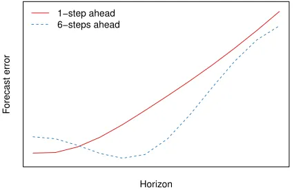
changing the parameter optimisation cost function. Figure 1 provides a stylised view of the

expected forecast errors, for a given model, that is optimised to best approximate 1-step

ahead behaviour or multiple steps ahead. The solid line that corresponds to the model

that is optimised to approximate 1-step ahead will have increasing forecast errors further

for longer horizons. On the other hand, the dashed line, corresponding to a model that is

optimised to approximate a 6-step ahead forecast, will have its best performance around

that forecast horizon, with poorer accuracy for shorter and longer horizons. In section 5,

we demonstrate this behaviour empirically using evidence from our retailing case study.

Therefore, by optimising the forecasting model parameters for different forecast horizons, we

attempt to overcome the approximate nature of the model to the data generating process

(Cox, 1961; Tiao and Xu, 1993; Chatfield, 2000).

Horizon

F

orecast error

1−step ahead 6−steps ahead

Figure 1: Stylised representation of the expected forecast errors of a model optimised on 1-step and 6-steps ahead errors. Figure 3 illustrates an empirical case.

This would be an intuitive ‘fix’ from a user perspective, but its modelling implications are

not researched thoroughly, for example, the effect on model parameters is unknown. This is

important as the model parameters directly afffect the forecast variance, i.e. its uncertainty,

and therefore the quality of the decisions supported by forecasting, such as inventory or

and therefore this is a general problem that needs to be addressed, wider than exponential

smoothing forecasts.

For producing up to h-step ahead forecasts, we investigate two approaches: i) build

h different models, each one optimised on the relevant steps-ahead in-sample error (for examples of this approach see: Tiao and Xu, 1993; Haywood and Tunnicliffe Wilson, 1997;

Clements and Hendry, 1998; Pesaran et al., 2011) and ii) build a single model and parametrise

it with what we nametrace optimisation, as it is based on the trace of forecasts over multiple

horizons, i.e. the forecasted values fromt+ 1 tot+h, combininghdifferent multi-step ahead cost functions (Weiss and Andersen, 1984).

Although these objective functions are not new in the literature, in this work, we show

that they equate to a type of univariate shrinkage that differs from existing shrinkage

ap-proaches, such as ridge and lasso regression (Hastie et al., 2009). Existing approaches

func-tion in a regression context, and therefore are unable to handle moving average terms,

that are the basis of many time series models, such as exponential smoothing and ARIMA.

Furthermore, they do not treat univariate information in a different way than explanatory

regressors, even though they are qualitatively different (Wang et al., 2007). This

univari-ate shrinkage reduces the potential overfit of the model to the data and therefore address

the limitation that the underlying process is unknown, similarly to conventional

shrink-age estimators (Tibshirani, 1996). We describe the nature of the achieved shrinkshrink-age and

provide empirical evidence of its effect on model parameters and demonstrate substantial

improvements in forecasting accuracy and economic costs. We provide empirical evidence

by modelling sales of different products in a supermarket chain. It should be noted that,

although we focus on the case of exponential smoothing, the insights developed here can be

extended to other univariate extrapolative forecasting models.

The rest of the paper is organised as follows: section 2 introduces the state space

expo-nential smoothing formulation and various alternatives for parameter estimation, leading to

univariate shrinkage. Section 4 presents the forecasting cases and the empirical evaluation

setup that will be used to demonstrate the shrinkage and the performance of the alternative

cost functions. Section 5 presents the results. We conclude with limitations of this univariate

shrinkage and this work, as well as directions for future research.

2. Exponential Smoothing Model

2.1. State space exponential smoothing model

Hyndman et al. (2002) embedded ETS within a state space framework, providing the

statistical rationale for the model. ETS is capable of modelling time series with different

types of trend: linear, damped or none; and seasonality. These may interact, together with

the error term, in an additive or multiplicative fashion, resulting in a total of 30 ETS model

forms, although in practice, typically, these are restricted to fewer forms (Kourentzes et al.,

2018).

The general exponential smoothing State Space approach can be expressed as follows

(Hyndman et al., 2008):

yt=w(xt−1) +r(xt−1)et, (1)

xt=f(xt−1) +g(xt−1)et. (2)

Equation (1) is known as the observation equation that relates the observation (yt) at timet with the state vectorxt−1. Such a vector contains unobserved components, more specifically

the level, trend and seasonality. Equation (2) is known as the state equation and describes

the evolution of states xt over time, while et is a white noise process with variance σ2 and zero mean. f(·) and g(·) are vector functions, whereasr(·) andw(·) are scalar functions.

The state vector in the general model is comprised by the level (lt), the trend (or slope

-bt) and seasonality unobservable states (st),xt = (lt, bt, st, st−1, . . . , st−m+1)0, wherem is the

errorr(xt−1) =µt, with µt=w(xt−1). That makes the observation equation (1)yt =µt+et and yt = µt(1 +et) for the additive and multiplicative error cases, respectively. The rest differ depending on the model form.

For example, for the well known local level model, ETS(A,N,N) that has an (A)dditive

er-ror term, (N)o trend and (N)o seasonality, and corresponds to the single exponential

smooth-ing method: xt = (lt),w = 1, f(xt−1) =xt−1 and g =α, where 0 < α <1 is the smoothing

parameter. This results in µt=lt and the well known:

yt=lt−1 +et, (3)

lt=lt−1 +αet. (4)

The forecast can be generated from the observation equation (3) as E(yn+h|n) = µn+h|xn,

which in turn givesft+h =lt. From the formulation above, it is apparent that large smoothing parameter α causes the level component, equation (4), to become very reactive to new information and vice-versa. For example, if α is close to 1 the level component behaves almost like a random walk.

Similarly for the local trend model, ETS(A,A,N) that corresponds to Holt’s exponential

smoothing method, with smoothing parameters g =

α β

0

and 0 < β < α, has a state space structure:

xt=

lt bt

0

, _{w(xt−1) =}

1 1

xt−1, f(xt−1) =



 

1 1

0 1



 xt−1.

This can be reformulated in the more usual form:

yt =lt−1+bt−1+et,

lt =lt−1+bt−1+αet,

Another common model is the seasonal variant ETS(A,N,A). The state vector has m

seasonality states, and m equals the seasonal periodicity. Let Ik denote thek ×k identity matrix, and 0k denote a vector of zeros of lengthk:

w(xt−1) =

1 00_m−1 1

xt−1, f(x_t−1) =

     

1 00_m−1 0

0 00_m−1 1

0m−1 I0m−1 0m−1

     

xt−1,

g(xt−1) =

α γ 0m−1

0

, where 0 < γ < 1−α is the smoothing parameter for the sea-sonality. The model can be written in the more familiar exponential smoothing formulation

as:

yt=lt+st−m+et

lt=lt−1 +αet

st=st−m+γet

Having described ETS(A,N,N), ETS(A,A,N) and ETS(A,N,A) we provide a brief overview

of how the different model components and parameters interact, which will be helpful in

understanding the effect of the alternative cost functions. The reader is referred to Hyndman

et al. (2008) for a description of the remaining ETS models.

2.2. Model estimation

The standard way to parametrise ETS is using maximum likelihood estimation.

Equiv-alently, we can minimise the augmented sum of squared error criterion:

S(θ,x0) = [exp(L(θ,x0))]1/n =

n Y t=1

r(xt−1)

2/n _n

X

t=1

whereθ are the model parameters,x0 the initial values of the state vector,L is the negative

log likelihood andn the fitting sample size.

Recall that for additive error modelsr(xt−1) = 1. Therefore, for ETS with additive error

using the augmented sum of squared criterion is the same as minimising the one-step ahead

in-sample Mean Squared Error (MSE):

MSE = 1

n

n

X

i=1

yi−yˆi|i−1

2

, (5)

where ˆyi|i−1 is the forecasted value for period i, conditioned on prior information. We will

refer to ETS parametrised using equation (5) as ETSt+1.

An alternative approach is to optimise the model using an h-step ahead loss, where h

matches the forecasting objective:

MSEh = 1

n−h+ 1 n

X

i=h

yi−yˆi|i−h

2

, (6)

where ˆyi|i−h is the forecast in period i from origin i−h. Observe that the number of errors that are used in the calculation of MSEh are less than the number for conventional one-step

ahead MSE by h−1. This approach was originally discussed for exponential smoothing by Cox (1961) and since has been further investigated in the literature, both in the context of

exponential smoothing and other models (for examples see: Tiao and Xu, 1993; Haywood

and Tunnicliffe Wilson, 1997; Clements and Hendry, 1998). Clements and Hendry (1998)

demonstrate that if the model parameters are estimated using the horizon in the cost function

that matches the forecast objective, then the loss of forecasting performance is small at longer

horizons, relative to shorter horizons, even if an incorrect model is used. This is not true for

the one-step ahead cost. This finding is intuitive, as it is expected that models parametrised

to match the forecasting objective should perform better, nonetheless the overwhelming

majority of models in both practice and the literature are optimised using one-step ahead

In practice, equation (6) implies that if we are interested in all horizons from 1 to h, then h models need to be estimated and each will be used separately to produce only the forecast of the relevant horizon. Each model will be parametrised to achieve an as good

as possible approximation for the target forecast horizon (see figure 1). As the forecast

trace, from t + 1 to t+h is composed by the outputs of h different models, there is no guarantee that the dynamics captured in the h different forecasts are similar. This can cause discontinuities in the forecasts and prediction intervals, as the horizon increases. For

example, consider the case of ETS(A,N,N), where for t+ 1 the forecast will be based on a different smoothing parameter than fort+h, and as such will have different values, in contrast to the conventionally expected forecast for ETS(A,N,N), i.e. the result of ETSt+1, that forms

a horizontal line across different horizons. Hereafter, we will refer to ETS parametrised using

equation (6) as ETSt+h.

In order to avoid parametrisinghseparate models, we can construct a hybrid cost function that attempts to match the multiple forecasting objectives: predicting all 1 toh-steps ahead as accurately as possible. To do that we construct the following cost function:

MSEtrace = 1

h

h

X

i=1

MSEh. (7)

Under this cost function the MSE of various different forecast horizons, as calculated using

equation (6), are combined using an unweighted average. The objective of the trace

opti-misation is to achieve on average a good fit across multiple horizons, instead of a single

one. To the best of our knowledge this approach has been used very sparsely in the

liter-ature. Weiss and Andersen (1984) discussed optimising using traces of forecasts and found

promising accuracy results. Hyndman et al. (2002) used it as an alternative parameter

es-timation cost function for ETS. However they did not elaborate on the rationale behind its

use and selected the average of 1 to 3 steps-ahead errors, even though the forecast horizons

of MSEtrace (referred as AMSE by Hyndman et al., 2002) did not match the forecast

ob-jective, it was still found to perform best over alternative parameter estimation approaches.

Xia and Tong (2011) investigated trace optimisation in more detail. With the aim to avoid

assuming that the postulated model is true, they construct a cost function that incorporates

several multiple-step ahead errors to fit a model to a time series. However, they do not use it

primarily for forecasting tasks. They argue that their approach maximises feature matching,

i.e. given the knowledge that the model that is used is not true, they address the question of

how to best tune a model to fit the observed features of a time series, and therefore use it to

understand and characterise the processes in time series. In agreement with the results by

Hyndman et al. (2002), they find that models optimised in this way fit and describe better

their data, in particular for medium to long horizons.

Trace optimisation does not require building multiple forecasting models, as is the case

for ETSt+h, but requires more computations than the conventional ETSt+1, as at each

in-sample forecast origin we need to construct trace forecasts. For the rest of this paper we will

refer to the ETS parametrised with trace optimisation as ETStrace.

Note that the cost functions discussed here are not exclusive to ETS and could be used

with any forecasting model. In this work, we focus to ETS as it is a well established and

understood forecasting model that at the same time is simple and easy to implement in

practice and it is widely available in forecasting software. Furthermore, the cost functions

above could be constructed with different than the quadratic loss, if desired. Finally, all

model parameters, in this case the α controlling the local level, the β controlling the local slope, the γ controlling the local season, the φ controlling the dampening of the slope and the initial parameters x0 of the exponential smoothing are optimised simultaneously, using

3. The connection of multi-step and trace optimisation with parameter shrinkage

In this section, we assume that the main term that governs the MSEh is the h-step

ahead forecast variance, which can be theoretically obtained from the forecasting model.

This assumption will allow us to interpret analytically the influence of trace optimisation on

parameter shrinkage. Later on, such an assumption will be empirically verified.

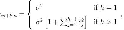
Based on the state space formulation, the forecast variance is given by

vn+h|n=

  

 

σ2 _{if h= 1}

σ2h_{1 +}Ph−1

j=1c 2

j

i

if h >1

, (8)

where cj depends on the model form and contains its parameters. Expressions for all linear homoscedastic and heteroscedastic exponential smoothing models exist. Table 1 lists the

cj values for some common models, where dj,m = 1 if j (mod m) is equal to zero and 0 otherwise. The reader is referred to Hyndman et al. (2008) for an exhaustive list.

Table 1: Value forcj

Model cj

ETS(A,N,N)/ETS(M,N,N) α

ETS(A,A,N)/ETS(M,A,N) α+βj

ETS(A,N,A)/ETS(M,N,A) α+γdj,m

From equation (8) and table 1 we can write the h-steps ahead variance of the forecast for ETS(A,N,N):

vn+h|n=σ2

1 +α2(h−1), (9)

whereσ2_{is the one-step ahead variance that is approximated as the in-sample one-step-ahead}

MSE, as in equation (5). From equation (9) it is clear that the variance increases as the

not affected by the shrinkage.

At this point, it is helpful to consider the nature of parameter shrinkage. Using

equa-tion (9) as an example, we can see that as the forecast horizon h increases the smoothing parameter α of ETS(A,N,N) will be pushed towards zero. This will result in the local level

lt of the model to be updated less, as the term αet in equation (4) will have a lesser effect. Across forecast origins, this makes the forecast less volatile. The intuition behind this is that

since we do not expect the model to correctly capture the underlying demand process, we

lessen the effects of the terms of the model that may very well be misspecified. In contrast,

when α is not shrunk, that term fully affects the updating of the forecasts across origins. When the model does not match the data generating process, this will inappropriately

in-crease the variability of forecasts and harm its forecasting performance. This follows from

the logic of the bias-variance trade-off, where by shrinking parameters to zero we under-fit

to the in-sample data (increase model bias), to achieve better out-of-sample performance

(decrease model variance), given the risk that the model used does not match the underlying

dynamics (Hastie et al., 2009).

We can easily derive the cumulative variance for the trace forecast, i.e. the forecasts from

t+ 1 up to h-steps ahead:

Vn+h|n = h

X

j=1

vn+j|n

= h

X

j=1

σ2

1 +α2(j−1)

. (10)

Bearing in mind that Ph

j=1j = 1

2h(h+ 1), we can rewrite equation (10) as:

Vn+h|n=hσ2+α2

h

2(h−1)σ

2_{. (11)}

Again, in equation (11) the impact of α increases with h, but the weight of the smooth-ing parameter on σ2 _{increases by the number of forecasts included in the trace, making}

the shrinkage more pronounced than before. Therefore, small increases in the smoothing

Using the same logic, we can easily derive the variances for the local trend ETS from

table 1. It is interesting to investigate the behaviour of the seasonal model due to the effect

of dj,m. The h-step ahead variance is:

vn+h|n =σ2

1 +α2(h−1) +γhm(2α+γ)

, (12)

where hm is the number of complete years in the forecast period:

hm =

(h−1)

m

. (13)

Using equations (12) and (13) we can rewrite the h-step ahead variance as:

vn+h|n=σ2+α2(h−1)σ2 + (2αγ+γ2)

(h−1)

m

σ2, (14)

where a similar behaviour to α is observed for γ. As the value of γ increases, variance increases as well. Therefore minimising the h-step ahead variance will result in shrinking bothαandγ. However, in contrast toα(andβ for the trend models) the effect ofγincreases in a stepwise manner, as controlled byhm, i.e. the shrinkage increases every complete season. In fact, when the forecast horizonhis less than the seasonal periodmno shrinkage is imposed on γ. Also, note that there is an interaction term between α and γ in the seasonal part of the variance expression.

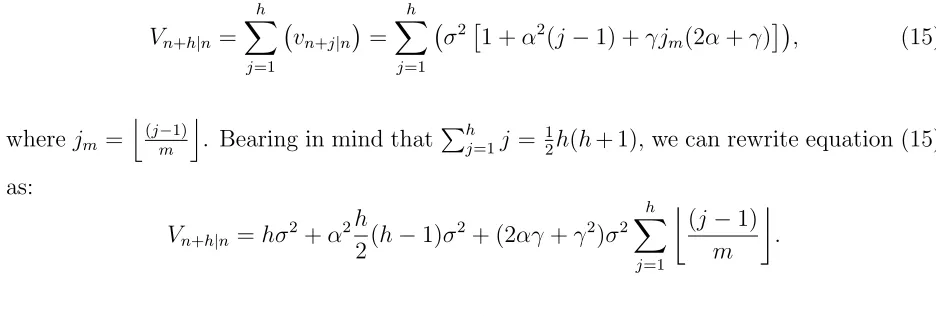
Similarly, we can write the cumulative variance for the trace forecast up toh-steps ahead:

Vn+h|n= h

X

j=1

vn+j|n

= h

X

j=1

σ21 +α2(j−1) +γjm(2α+γ)

, (15)

wherejm =

j

(j−1)

m

k

. Bearing in mind that Ph

j=1j = 1

2h(h+ 1), we can rewrite equation (15)

as:

Vn+h|n=hσ2+α2

h

2(h−1)σ

2_{+ (2αγ+γ}2_)σ2

h

X

j=1

(j−1)

m

As before, the impact of α increases with h, while γ and the interaction term increases in a stepwise manner. The weight of the smoothing parameters on σ2 _{increases by the}

number of forecasts included in the trace, making the shrinkage more pronounced than

before. Therefore, small increases in the smoothing parameters will have substantial impact

onVn+h|n.

In general, we find that the shrinkage of both α and β increases with h, although the latter shrinks faster thanα, while γ shrinks in a stepwise manner, increasing every complete season. As for the damped trend models, we find that parameterφ, which controls the degree of trend dampening, slows the shrinkage ofβ, given 0 < φ <1.

Another helpful example to better understand the effect of parameter shrinkage is to

consider the local linear trend model ETS(A,A,N). In this case, parameter shrinkage happens

faster forβthan forα. Shrinking itsβparameter towards zero, will bring the model closer to having a deterministic trend, effectively transforming the model to the very well performing

Theta method. This method has ranked top in past forecasting competitions (Makridakis and

Hibon, 2000), and has been shown to be equivalent to an ETS(A,N,N) with a deterministic

trend component (Hyndman and Billah, 2003).

We anticipate that the additional shrinkage imposed by the trace optimisation will make

the error surface of the trace error steeper than both conventional one-step ahead

optimisa-tion and h-steps ahead, as the parameters will have to overcome additional shrinkage. To explore this further we consider the gradients of vn+h|n and Vn+h|n with respect to α for

h≤m:

∂vn+h|n

∂α =σ

2_2α(h−1),

∂Vn+h|n

∂α =σ

2_αh(h−1).

than the one provided by the h-steps ahead cost function, and this additional steepness depends on the forecast horizon.

The discussion in this section shows that the use of multi-step or trace forecasts in the

cost function results in parameter shrinkage. This introduces the notion of shrinkage for

exponential smoothing, which so far has been mostly applied to regression type models

(Hastie et al., 2009). Thus, we avoid the introduction of ad-hoc parameter constraints

or manual overrides that are common in practice and whose effect is ill-understood, often

resulting in parameter values on bounds imposed by the ad-hoc introduced constraints. In

contrast, here we describe the magnitude and direction of the proposed shrinkage mechanism.

Note that the trace cost function, as defined in (7), does not consider the possible

covari-ances between multi-step errors. Chatfield (2000) argues that even when empirical errors

may demonstrate covariances, the simplified theoretical variance formulas can provide

in-sights into the general case, for which we conjecture that similar shrinkage behaviour will be

observed.

4. Empirical evaluation setup

In this section, we provide the setup of the empirical evaluation, along with an overview

of the data used and the evaluation criteria.

4.1. Datasets

We use a collection of seven datasets that describe sales for different product types

across different retail stores of a supermarket chain. Predicting sales is a common objective

in business forecasting applications and we refer the reader to past work in retail forecasting

for an overview of the specific challenges (Huang et al., 2014; Kourentzes and Petropoulos,

2016; Fildes et al., 2019). In this particular case, we are interested in constructing baseline

forecasts, which will be further adjusted to incorporate special events, as is the norm (Fildes

In total, we explore 7 types of products: cheese; dairy; frozen; grocery; fresh meat;

frozen meat; and a special category containing the most valued products for each store

(MVP), across 104 different stores, totalling in 728 daily time series, of variable length from

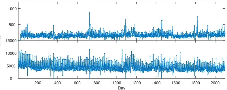
1021 to 3360 observations. Figure 2 provides a sample sales series, where the

complex-ity is evident with prominent seasonalcomplex-ity, potential level shifts and other dynamics. The

data originate from the Dominick’s dataset, provided by James M. Kilts Center,

Univer-sity of Chicago Booth School of Business (http://research.chicagogsb.edu/marketing/

databases/dominicks/).

500 1000

Sales

200 400 600 800 1000 1200 1400 1600 1800 2000

Day

0 5000 10000 15000

Figure 2: Examples of cheese sales from two supermarket stores.

4.2. Experimental design

The data is separated into two subsets, the first is used to estimate the models and the

second to evaluate their out-of-sample performance. The last half year of data (192 days) is

used as a test set and the forecast horizon is set to 7 days.

We use relatively long test sets to produce a large number of forecasts, over the different

phases of the year, ensuring a rigorous evaluation. Once a forecast is produced, the forecast

origin is shifted by one period ahead and the process is repeated until there is no more test

set sample. In total 186 forecast traces are produced and used to evaluate the different cost

functions, for each time series. A detailed description of the rolling origin evaluation scheme

4.3. Evaluation metrics

4.3.1. Forecast metrics

In measuring the forecast accuracy, we are interested to summarise the results across

multiple stores and product types. To this end, we use the Average Relative Mean Absolute

Error (AvgRelMAE), proposed by Davydenko and Fildes (2013). The advantage of this

metric is that it has desirable statistical properties, and provides reliable aggregate figures

when summarising over diverse time series. It is calculated as:

MAEh = 1

T

T

X

t=1

|yt+h −yˆt+h|,

AvgRelMAE_h = N

v u u t

N

Y

i=1

MAEh,A,i MAEh,B,i

,

where yt+h and ˆyt+h stand for the actual value and the forecast of horizon h from origin t, respectively, at time t +h, for all periods T in the test set. MAEh,A,i and MAEh,B,i are the Mean Absolute Errors (MAE) of the forecast considered (A) and the benchmark (B),

for a given h and time series i = 1, . . . , N. As a benchmark, we use the conventionally optimised exponential smoothing. If the resulting AvgRelMAE is below one, then the

fore-cast of interest is more accurate than the benchmark. We can also interpret AvgRelMAE

as percentage improvement from the benchmark by calculating (1−AvgRelMAE)×100%.

We summarise the results further by considering the geometric mean of AvgRelMAE across

forecast horizons.

4.3.2. Economic metrics

In addition to the forecast comparison metrics, this section assesses the monetary benefits

of the considered loss functions. An economic metric that is typically used in a supply chain

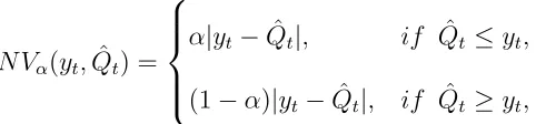
context is the news-vendor cost (NV), also known as the tick-loss or pinball cost and it can

N Vα(yt,Qˆt) =

   

  

α|yt−Qˆt|, if Qˆt≤yt,

(1−α)|yt−Qˆt|, if Qˆt≥yt,

(16)

of order α ∈ (0,1), where any α-quantile of the predictive distribution is an optimal point forecast (Gneiting, 2011), i.e. it minimises the newsvendor cost function. ˆQt is the quantile forecast. In the supply chain literature, the target quantile α is given by the Cycle Service Level (CLS, Silver et al., 2017). The CSL expresses the asymmetry in cost terms, such as

CSL = Ca

Ca+Cb (Gneiting, 2011), where Cb and Ca are the cost of over-forecasting ( ˆQt > yt)

and under-forecasting ( ˆQt < yt), respectively. For example, a value of CSL = 0.9 means that the under-forecasting cost is 9 times the over-forecasting cost. Often, practitioners prefer

using CSL interpretation instead of under- or over-forecasting costs, because the estimation

of Ca, which is related to the stock-out cost, may not be available.

To compute the economic impact of forecasts, we need the lead time quantiles, ˆQL(CSL), for a determined target CSL:

ˆ

QL(CSL) = ˆyL+k(CSL)ˆσL (17)

where k = Φ−1(CSL) is the safety factor and Φ(·) denotes the standard normal cumulative distribution function. The ˆyL=PL_j=1yˆt+j is the lead time point forecast and ˆσL is the lead time standard deviation forecast, given by:

ˆ

σ2_L=σ2

L−1

X

j=0

C_j2, (18)

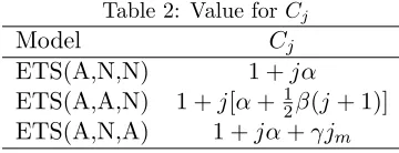
where Cj values can be found in (Hyndman et al., 2008, p. 91). Table 2 provides the matching expressions for the model forms introduced in section 3.

Table 2: Value forCj

Model Cj

ETS(A,N,N) 1 +jα

ETS(A,A,N) 1 +j[α+1₂β(j+ 1)]

ETS(A,N,A) 1 +jα+γjm

terms of both point (ˆyL) and variance forecasts (ˆσL).

To summarise the results and to avoid unit differences presented due to the scale of the

datasets analysed, we compute a cost ratio as the quotient of the NV cost provided byET St+h or ET Strace with respect to standard practice ET St+1. This matches the interpretation of

AvgRelMAE used of the forecast evaluation. The lead times analyzed vary from 1 to 7,

and the target CSLs are set to 0.5, 0.6, 0.7, 0.8 and 0.9. In addition, σ is estimated using only the in-sample data, retaining a clear separation with the test set, where the NV cost is

calculated.

4.4. Exponential Smoothing

Exponential smoothing (ETS) has been used successfully to forecast retailing sales in

multiple cases (Gardner, 2006; Kourentzes and Petropoulos, 2016; Fildes et al., 2019). The

exponential smoothing family of models can successfully capture level, trended and

sea-sonal time series. We use ETS as embedded within the state space framework (Hyndman

et al., 2002), which permits selecting between the various model forms using an appropriate

information criterion, such as Akaike’s Information Criteria (AIC) that we use here.

We evaluate all three alternatives in estimating the parameters of the model, as outlined

in section 2.2, (i) conventionally, i.e. t+ 1; (ii) for each forecast horizon separately; and (iii) using the trace forecast from t+ 1 up to t+ 7. These are named, in the same order, as: ETSt+1, ETSt+h and ETStrace. Note that, to correctly use AIC for model selection the

model parameters must maximise its likelihood. Therefore, model selection is done when

ETS parameters are optimised in the conventional way and the same model is retained for

5. Results

We have organised the results of our empirical evaluation into separate subsections,

dis-cussing forecast accuracy gains, evidence of the univariate shrinkage, cost implications for

our case study and concluding with some remarks on computational efficiency.

5.1. Forecast accuracy

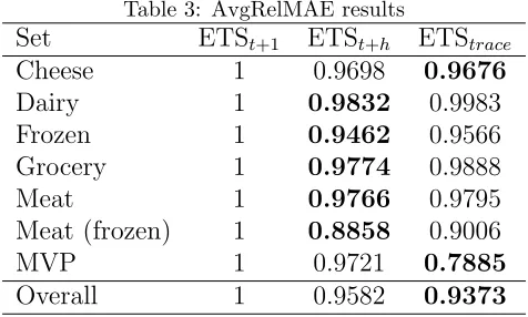
Table 3 provides the overall AvgRelMAE performance for the seven sets of products. In

each row, the approach with the lowest forecast error is highlighted in boldface. The accuracy

for ETSt+1 is used as the benchmark in the calculation of AvgRelMAE, and therefore it is

always reported as 1.

Table 3: AvgRelMAE results

Set ETSt+1 ETSt+h ETStrace

Cheese 1 0.9698 0.9676

Dairy 1 0.9832 0.9983

Frozen 1 0.9462 0.9566

Grocery 1 0.9774 0.9888

Meat 1 0.9766 0.9795

Meat (frozen) 1 0.8858 0.9006

MVP 1 0.9721 0.7885

Overall 1 0.9582 0.9373

We can observe that in all cases both ETSt+h and ETStrace outperform the benchmark.

Overall the gains are close to 4% for ETSt+h and 6% for ETStrace, although the difference is

mainly driven by the notably better accuracy on the MVP set of products. The differences

are found to be statistically significant at 1% level, using the non-parametric Friedman and

post-hoc Nemenyi tests (Hollander et al., 2013).

Figure 3 presents the AvgRelMAE per horizon across all sets of products. The

perfor-mance of the benchmark ETSt+1, which is the standard practice, is always equal to 1. We

can observe that, for forecast horizon t+ 1 ETSt+h is identical to the benchmark, since at this horizon the two approaches are optimised identically. ETStraceis marginally worse. This

t+1 t+2 t+3 t+4 t+5 t+6 t+7 Horizon

0.86 0.88 0.9 0.92 0.94 0.96 0.98 1 1.02

AvgRelMAE

ETS_t+h

ETS_trace

Figure 3: Overall AvgRelMAE of ETSt+h and ETStrace across forecast horizons.

error. As the horizon increases, the gains of ETSt+h and ETStrace become evident, with the

latter being for the remaining forecast horizons the most accurate. Observe that close to the

horizont+ 7 the gains are smaller than in the preceding forecast horizons. This is explained by the majority of the sales series being seasonal. The seasonal periodicity is 7 days, and

therefore at to the completion of the seasonal cycle the observed level of the time series is

somewhat similar to the level observed at the forecast origin, making the benchmark ETSt+1

relatively more accurate.

The unknown data generating process of the retail sales series is only approximated by

the exponential smoothing family of models, omitting multiple drivers and shocks, such as

promotions, that occur in practice. Therefore, the expectation that conventional likelihood

estimation will result in appropriate parameters does not hold. The resulting model is merely

parametrised so as to have low one-step ahead error. If the model was correcting capturing

the underlying process, then the likelihood estimated parameters would be sufficient, but this

assumption of model ‘trueness’ hardly holds in practice. The empirical evidence supports

our argument that this approach leads to predictive models that are myopically tuned for

horizon, therefore we avoid focusing only on the short horizons. The prediction for each

horizon is tuned specifically for that, thus helping the model to approximate the retail sales

for all requested horizons. The results of the empirical evaluation demonstrate that this

strategy performs very well, resulting in accurate predictions. However, this comes at the

cost of parametrising 7 separate models, one for each forecast horizon. There is a trade-off

between computational cost and lifting the assumption that the employed model is true.

The ETStrace is attempting to bridge the two extremes. Only a single model is fitted to

the data, hence keeping the computational cost low. Moreover, the objective of the model is

to be accurate at all forecasting horizons (from 1 to 7 hours ahead), with equal importance.

In practice, the resulting forecasts are not optimally tuned for any forecast horizon, yet, at

the same time, the model is not over-fit for any, resulting in good overall performance.

5.2. Parameter shrinkage

We turn our attention to the estimated model parameters. Our theoretical argument

was that, we expect to observe shrinkage of the smoothing parameters for ETSt+h and

ETStrace. More specifically, since we focus on forecast horizons up to the seasonal length,

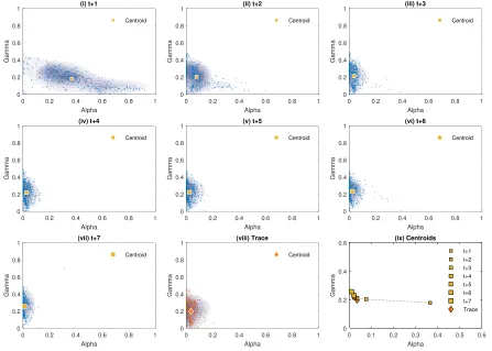
this effect should not be observed for the γ smoothing parameter that is connected to the seasonality. Figure 4 plots the parameters for all seasonal ETS(A,N,A) models across all 728

time series. We focus on ETS(A,N,A) as it is the selected model for 63.3% of the cases and

has two smoothing parameters, namelyαassociated to the local level andγ associated to the seasonality, which allows for informative plots. The figure has 9 subplots. The first seven,

(i)–(vii), plot the parameters for models optimised on 1 to 7-steps ahead. Each plot provides

the combination of fitted parameters for each time series, a density cloud to highlight the

concentration of points, and the centroid. Subplot (vii) provides the same information for

the resulting parameters for ETStrace, while the last subplot (ix) plots only the centroids to

clearly show how they change for the different cost functions. The size of the marker used

to represent the centroid increases in size with the forecast horizon.

0 0.2 0.4 0.6 0.8 1 Alpha 0 0.2 0.4 0.6 0.8 1 Gamma (i) t+1 Centroid

0 0.2 0.4 0.6 0.8 1

Alpha 0 0.2 0.4 0.6 0.8 1 Gamma (ii) t+2 Centroid

0 0.2 0.4 0.6 0.8 1

Alpha 0 0.2 0.4 0.6 0.8 1 Gamma (iii) t+3 Centroid

0 0.2 0.4 0.6 0.8 1

Alpha 0 0.2 0.4 0.6 0.8 1 Gamma (iv) t+4 Centroid

0 0.2 0.4 0.6 0.8 1

Alpha 0 0.2 0.4 0.6 0.8 1 Gamma (v) t+5 Centroid

0 0.2 0.4 0.6 0.8 1

Alpha 0 0.2 0.4 0.6 0.8 1 Gamma (vi) t+6 Centroid

0 0.2 0.4 0.6 0.8 1

Alpha 0 0.2 0.4 0.6 0.8 1 Gamma (vii) t+7 Centroid

0 0.2 0.4 0.6 0.8 1

Alpha 0 0.2 0.4 0.6 0.8 1 Gamma (viii) Trace Centroid

0 0.1 0.2 0.3 0.4 0.5 0.6 Alpha 0 0.2 0.4 0.6 Gamma (ix) Centroids t+1 t+2 t+3 t+4 t+5 t+6 t+7 Trace

Figure 4: Scatter plots of smoothing parameters of ETSt+h, subplots (i)–(vii), and ETStrace, subplot (viii).

across a wide range of values, with many of them being very high. When the exponential

smoothing α value is high, the recent observations receive the highest weights, whereas the weight of older observations decay exponentially over time. This implies that the estimated

model is very reactive to changes in the level, with α = 1 assuming a random walk model for the level of the time series. This often over-interprets noise in the time series as useful

level information. To avoid this, in the literature, it has been suggested to constrain the

parameters to values below 0.5 (for example, Johnston and Boylan, 1994), although such

restrictions are ad-hoc and may not result in maximum likelihood estimates. Given that the

seasonal component of ETS is based on the level estimation, a high α parameter may harm accuracy further. We observe that the mean of the α is just below 0.4, as indicated by the centroid. The γ values range between (0,0.4].

As the forecast horizon considered in the cost function increases in the following

sub-plots (ii)–(vii), we observe that the values of α are gradually shrunk, towards zero. The shrinkage becomes stronger for longer horizons, as our theoretical analysis indicated. The

low smoothing parameter values imply a very persistent level, resistant to local disturbances

that exponential smoothing is unable to capture. Furthermore, this assists the estimation

of the seasonal component. All these factors contribute to the increased forecast accuracy

observed for ETSt+h, evident in Table 3 and Figure 3. On the other hand, the γ parameter remains in the same range of values, as expected, since it is not subject to shrinkage.

The evolution of the shrinkage for α is also evident in subplot (ix) that provides the centroids for each cost function. We can see that, as the forecasting step increases, the

mean value of α monotonically decreases, matching the insights from (14), where for longer forecast horizons the shrinkage is more pronounced.

Subplot (viii) provides the estimated parameters for ETStrace. It is evident from the

ort+ 7 horizons. Consulting subplot (ix), we observe that the centroid for ETStrace is close to the centroids for t+ 3 andt+ 4.

These observations are in agreement with the shrinkage interpretation for ETSt+h and

ETStrace, where the α smoothing parameter quickly shrinks to small values as h increases, whereas the step-wise nature of hm limits the shrinkage of γ. In fact, in our evaluation that considers h ≤ m, the term hm = 0 and, therefore, no shrinkage of γ is done and hence the observed parameter behaviour.

For brevity, we do not provide plots of the smoothing parameters of the other models

fitted to the remaining time series (these were ETS(A,N,N), ETS(A,Ad,N), ETS(A,A,A)

and ETS(A,Ad,A), for 1.92%, 0.14%, 1,1% and 33.52% of the series respectively, apart from

the already reported ETS(A,N,A)), as their behaviour is similar and matches the theoretical

understanding from section 3.

5.3. Inventory cost

The economic impact of the forecast accuracy improvement is measured through the

cost ratio associated with the news-vendor cost over the lead time for a determined CSL,

N Vcsl(yL,QˆL), introduced in (16).

Figure 5 shows the cost ratio versus lead time for each dataset. This cost ratio has

been averaged across target CSLs. In 6 out of 7 datasets, ETSt+h obtains a lower cost than

the benchmark ETSt+1 for every lead time greater than 1, since for h = 1 both results are

the same. The biggest improvement is achieved for the Meat (frozen) dataset, where the

cost ratio is close to 0.7, indicating a 30% cost reduction. For ETStrace we observe that,

depending on the dataset, it outperforms ETSt+1 for medium to longer lead times. This

is not too dissimilar to the forecast accuracy findings, summarised in Figure 3, where for

t+1 ETStrace was found to be less accurate than the benchmark. Furthermore, for longer

lead times the performance of ETStrace becomes closer to that of ETSt+h. In the case of

the grocery dataset, ETStrace performs marginally better than ETSt+h for lead times of 4 or

where ETSt+hexhibits the best performance across all lead times, while ETStraceoutperforms

the benchmark ETSt+1 for lead times longer than 3.

2 4 6

Lead time 0.8 0.85 0.9 0.95 1 Cost ratio Cheese

2 4 6

Lead time 1 1.05 1.1 Cost ratio Dairy

2 4 6

Lead time 0.85 0.9 0.95 1 Cost ratio Frozen

2 4 6

Lead time 0.9 0.95 1 Cost ratio Grocery

2 4 6

Lead time 0.9 0.95 1 1.05 Cost ratio Meat

2 4 6

Lead time 0.8 0.9 1 1.1 1.2 Cost ratio Meat (frozen)

2 4 6

Lead time 0.95 1 1.05 Cost ratio MVP

2 4 6

Lead time 0.9 0.95 1 1.05 Cost ratio Average ETS t+h ETS trace

Figure 5: Cost ratio of ETSt+h and ETStrace per dataset versus lead times. The last subplots provides the

average cost ratio across all datasets.

Figure 6 shows the achieved cost ratio per dataset for different target CSLs. In most of

the datasets (6 out of 7) ETSt+h and ETStraceoutperform ETSt+1. The biggest improvement

is observed in the Meat (frozen) dataset, with a 25% and 20% cost reduction for ETSt+h and

all datasets. Although the most significant cost ratio improvements occur for a target CSL

of 50%, we observe gains throughout the range of CSLs, with the cost ratio always being

under 1, i.e. improving over the benchmark ETSt+1.

0.5 0.6 0.7 0.8 0.9

Target CSL 0.75 0.8 0.85 0.9 0.95 1 Cost ratio Cheese

0.5 0.6 0.7 0.8 0.9

Target CSL 0.95 1 1.05 1.1 1.15 1.2 Cost ratio Dairy

0.5 0.6 0.7 0.8 0.9

Target CSL 0.9 0.92 0.94 0.96 0.98 1 Cost ratio Frozen

0.5 0.6 0.7 0.8 0.9

Target CSL 0.9 0.92 0.94 0.96 0.98 1 Cost ratio Grocery

0.5 0.6 0.7 0.8 0.9

Target CSL 0.9 0.92 0.94 0.96 0.98 1 Cost ratio Meat

0.5 0.6 0.7 0.8 0.9

Target CSL 0.7 0.8 0.9 1 Cost ratio Meat (frozen)

0.5 0.6 0.7 0.8 0.9

Target CSL 0.95 0.96 0.97 0.98 0.99 1 Cost ratio MVP

0.5 0.6 0.7 0.8 0.9

Target CSL 0.9 0.92 0.94 0.96 0.98 1 Cost ratio Average ETS_t+h ETS_trace

Figure 6: Cost ratio of ETSt+hand ETStraceper dataset versus target cycle service levels. The last subplots

provides the average cost ratio across all datasets.

5.4. Computational implications

The final aspect of our analysis of the experimental results focuses on the computational

the models for each time series, and divided that by the time required to optimise the

benchmark model that uses only one-step ahead errors. The relative computational times

were summarised using the geometric mean, to find that ETSt+h required 7.36 times more,

while ETStrace required only 0.97 times. In fact, the latter has no significant difference in

terms of computational time with ETSt+1 (Wilcoxon test p-value is 0.709).

The substantial computational cost of ETSt+h is due to the need to estimate h models, 7 for our case. Note that, in cases where the complete forecast trace is not needed, then

ETSt+h would be more competitive. ETStrace requires more calculations than ETSt+1, but

as argued in section 3, it also results in steeper error surfaces, on which most optimisers

converge with fewer iterations.

6. Conclusions

Exponential smoothing is a very well established and researched model. In this work,

we focused on parameter estimation. When we use the conventional approach, of one-step

ahead estimators, we implicitly assume that the used exponential smoothing model is true

for the time series being modelled, i.e. models the underlying data generating process. This

is a very strong assumption, which when violated can result in poor forecasting accuracy for

multi-step predictions, something that has been observed multiple times in practice and the

literature. Naturally, poor forecasts harm subsequent decisions that rely on them.

The intuitive rationale for switching to multi-step or trace optimisation of model

param-eters is to match the forecast objective with the cost function. In our analysis, we show

that these are effectively shrinkage estimators, providing the statistical motivation for using

them. We describe fully the nature and size of the shrinkage and the insights from the

theoretical investigation match our empirical findings. Note that, the shrinkage described

here is different to the typical shrinkage used in a regression context, such as ridge and

LASSO. Although these have shown their strength in estimating coefficients of regressors

apparent if we consider the equivalences between exponential smoothing and ARIMA. Not

only exponential smoothing typically corresponds to integrated moving average processes,

but also implies several restrictions on the estimated parameters (exponential distribution

of weights, if the weighted moving average interpretation is used). These cannot be satisfied

by ridge or LASSO type shrinkage. On the other hand, for the same reasons, we argue that

the univariate shrinkage described here is not exclusive to exponential smoothing. It can be

extended easily to ARIMA models or any state-space model with some persistence vector g.

Therefore, multi-step and trace optimisation impose a new type of univariate shrinkage, the

strength of which is controlled by the forecast horizon.

In our empirical evaluation, we used exponential smoothing to produce forecasts for retail

sales. We find forecast accuracy gains and validate the theoretical arguments for parameter

shrinkage. These gains are matched by lower inventory costs, demonstrating economic gains

due to this parameter shrinkage. Overall, we find that both ETSt+h and ETStraceoutperform

substantially the conventional maximum likelihood estimation. Our results are interesting

for practice, since the cost functions discussed here can make ETS, a widely available model

in forecasting systems, perform very well. The implied shrinkage makes the forecasts less

sensitive to model and sample uncertainty. Although we provide here an evaluation of the

economic benefits of the resulting forecasts, future work should investigate in detail at the

impact of these cost functions on the prediction intervals of the forecasts.

However the gains from ETSt+h come at a computation cost, due to the large number

of models that need to be parametrised. In some applications, such as retailing, where the

required number of forecasts can be very large, this can be prohibitive (Seaman, 2018).

On the contrary, ETStrace, that demonstrated similar performance, requires building only

a single model. In our analysis we found that trace optimisation did not require more

computational resources than conventional optimisation, due to the steeper error surfaces

caused by the cost function. Therefore, we argued that ETStraceretains the desirable features

and produced consistent individualh-step ahead forecasts, without any abrupt changes that may be introduced by the h different models implied by ETSt+h, with advantages when calculating prediction intervals, but also simplifying its use by analysts.

A limitation that one should keep in mind is that the multi-step cost functions will result

in a smaller number of in-sample errors. This may be important for low sampling frequency

time series that may not have long histories, particularly when h becomes relatively long. For higher frequency time series, such as the ones used here, this is not relevant as the

estimation sample size is typically adequate, even when h−1 observations are lost. The exact implications of this for low frequency time series, as well as investigating theoretical or

empirical cut-off points for using multi-step ahead cost functions, are interesting questions

for future research.

We argue that it is fairly easy to adopt these cost functions in practice. Most forecasting

software, either standalone or as part of some ERP solution, offer some degree of

optimisa-tion for the parameters of the forecasting models. If the implementaoptimisa-tion is flexible enough

to provide control of the cost function to the user, then it would simply require enhancing

that aspect. However, many established software do not provide this option, but instead

allow setting parameters manually. In those cases, the analyst may decide to calculate any

model parameters externally and input those to the system. As the forecasting model

equa-tions remain the same, it can directly take advantage of the preset parameters, without any

additional changes. More flexible implementations that are based on forecasting packages

available for R, Python and other statistical computing languages, that are nowadays

in-creasingly embraced by industry, allow the flexibility for directly implementing these cost

functions to existing forecasting routines.

Finally, the insights for the multi-step and trace cost functions are applicable to other

time series models, such as ARIMA. Exploring this further is a promising research direction,

in particular, given that this type of shrinkage is of a different nature to typical shrinkage

with ridge and LASSO is appropriate. For example, using ridge or LASSO type shrinkage

can violate the ARIMA parameter conditions. This work offers a route forward for hybrid

shrinkage schemes that are appropriate both for univariate and explanatory inputs. It should

be noted that there is a fundamental difference between the specification of the two shrinkage

approaches. For the one discussed here, we cannot control the magnitude of shrinkage, as

this is fully depended on the forecast horizon. This simplifies modelling, which could be

considered an advantage, but at the same time loses the flexibility of reducing the shrinkage

effect when the used forecasting model is in fact close to the true underlying process.

References

Athanasopoulos, G., Hyndman, R. J., Kourentzes, N., Petropoulos, F., 2017. Forecasting

with temporal hierarchies. European Journal of Operational Research 262 (1), 60–74.

Barrow, D., Kourentzes, N., 2016a. The impact of special days in call arrivals forecasting:

A neural network approach to modelling special days. European Journal of Operational

Research.

Barrow, D. K., Kourentzes, N., 2016b. Distributions of forecasting errors of forecast

com-binations: implications for inventory management. International Journal of Production

Economics 177, 24–33.

Box, G. E. P., Jenkins, G. M., Reinsel, G. C., 1994. Time series analysis: Forecasting and

Control. Vol. 3rd. Prentice Hall Inc., New Jersey.

Chatfield, C., 2000. Time-series forecasting. CRC Press.

Clements, M., Hendry, D., 1998. Forecasting economic time series. Cambridge University

Press.

Cox, D. R., 1961. Prediction by exponentially weighted moving averages and related methods.

Davydenko, A., Fildes, R., 2013. Measuring forecasting accuracy: The case of judgmental

adjustments to SKU-level demand forecasts. International Journal of Forecasting 29 (3),

510–522.

Dietvorst, B. J., Simmons, J. P., Massey, C., 2015. Algorithm aversion: People erroneously

avoid algorithms after seeing them err. Journal of Experimental Psychology: General

144 (1), 114.

Fildes, R., Goodwin, P., Lawrence, M., Nikolopoulos, K., 2009. Effective forecasting and

judgmental adjustments: an empirical evaluation and strategies for improvement in

supply-chain planning. International journal of forecasting 25 (1), 3–23.

Fildes, R., Ma, S., Kolassa, S., et al., 2019. Retail forecasting: research and practice. Tech.

rep., University Library of Munich, Germany.

Gardner, E. S., 2006. Exponential smoothing: The state of the art, Part II. International

Journal of Forecasting 22, 637–666.

Gardner, Jr., E. S., 1988. A simple method of computing prediction intervals for time series

forecasts. Management Science 34 (4), 541–546.

Gneiting, T., 2011. Quantiles as optimal point forecasts. International Journal of Forecasting

27 (2), 197 – 207.

Hastie, T., Tibshirani, R., Friedman, J., Hastie, T., Friedman, J., Tibshirani, R., 2009. The

elements of statistical learning. Springer.

Haywood, J., Tunnicliffe Wilson, G., 1997. Fitting time series models by minimizing

multistep-ahead errors: a frequency domain approach. Journal of the Royal Statistical

Society: Series B (Statistical Methodology) 59 (1), 237–254.

Hollander, M., Wolfe, D. A., Chicken, E., 2013. Nonparametric statistical methods. Vol. 751.

Holt, C. C., 2004. Author’s retrospective on “Forecasting seasonals and trends by

exponen-tially weighted moving averages”. International Journal of Forecasting 20 (1), 11–13.

Huang, T., Fildes, R., Soopramanien, D., 2014. The value of competitive information in

forecasting fmcg retail product sales and the variable selection problem. European Journal

of Operational Research 237 (2), 738–748.

Hyndman, R. J., Billah, B., 2003. Unmasking the theta method. International Journal of

Forecasting 19 (2), 287–290.

Hyndman, R. J., Koehler, A. B., Ord, J. K., Snyder, R. D., 2008. Forecasting with

Expo-nential Smoothing: The State Space Approach. Springer-Verlag, Berlin.

Hyndman, R. J., Koehler, A. B., Snyder, R. D., Grose, S., 2002. A state space framework

for automatic forecasting using exponential smoothing methods. International Journal of

Forecasting 18 (3), 439–454.

Johnston, F. R., Boylan, J. E., 1994. How far ahead can an EWMA model be extrapolated?

The Journal of the Operational Research Society 45 (6), 710–713.

Kolsarici, C., Vakratsas, D., 2015. Correcting for misspecification in parameter dynamics to

improve forecast accuracy with adaptively estimated models. Management Science 61 (10),

2495–2513.

Kourentzes, N., Athanasopoulos, G., et al., 2018. Cross-temporal coherent forecasts for

aus-tralian tourism. Tech. rep., Monash University, Department of Econometrics and Business

Statistics.

Kourentzes, N., Barrow, D., Petropoulos, F., 2019. Another look at forecast selection and

combination: evidence from forecast pooling. International Journal of Production

Kourentzes, N., Petropoulos, F., 2015. Forecasting with multivariate temporal aggregation:

The case of promotional modelling. International Journal of Production Economics.

Kourentzes, N., Petropoulos, F., 2016. Forecasting with multivariate temporal aggregation:

The case of promotional modelling. International Journal of Production Economics 181,

145–153.

Kourentzes, N., Petropoulos, F., Trapero, J. R., 2014. Improving forecasting by estimating

time series structural components across multiple frequencies. International Journal of

Forecasting 30 (2), 291–302.

Makridakis, S., Hibon, M., 2000. The M3-competition: results, conclusions and implications.

International Journal of Forecasting 16 (4), 451–476.

Meese, R., Geweke, J., 1984. A comparison of autoregressive univariate forecasting

proce-dures for macroeconomic time series. Journal of Business & Economic Statistics 2 (3),

191–200.

Nenova, Z. D., May, J. H., 2016. Determining an optimal hierarchical forecasting model based

on the characteristics of the data set: Technical note. Journal of Operations Management

44, 62 – 68.

Ord, J. K., Fildes, R., Kourentzes, N., 2017. Principles of Business Forecasting, 2nd Edition.

Wessex Press Publishing Co.

Pesaran, M. H., Pick, A., Timmermann, A., 2011. Variable selection, estimation and inference

for multi-period forecasting problems. Journal of Econometrics 164 (1), 173–187.

Petropoulos, F., Kourentzes, N., Nikolopoulos, K., Siemsen, E., 2018. Judgmental selection

of forecasting models. Journal of Operations Management.

Pollack-Johnson, B., 1995. Hybrid structures and improving forecasting and scheduling in

Ritzman, L. P., King, B. E., 1993. The relative significance of forecast errors in multistage

manufacturing. Journal of Operations Management 11 (1), 51 – 65.

Sanders, N. R., Ritzman, L. P., 1995. Bringing judgment into combination forecasts. Journal

of Operations Management 13 (4), 311 – 321.

Seaman, B., 2018. Considerations of a retail forecasting practitioner. International Journal

of Forecasting.

Seifert, M., Siemsen, E., Hadida, A. L., Eisingerich, A. B., 2015. Effective judgmental

fore-casting in the context of fashion products. Journal of Operations Management 36, 33 –

45.

Silver, E., Pyke, D., Thomas, D., 2017. Inventory and Production Management in Supply

Chains. Fourth Edition. CRC Press. Taylor and Francis Group.

Sm˚aros, J., 2007. Forecasting collaboration in the european grocery sector: Observations

from a case study. Journal of Operations Management 25 (3), 702 – 716.

Taylor, J. W., 2007. Forecasting daily supermarket sales using exponentially weighted

quan-tile regression. European Journal of Operational Research 178 (1), 154 – 167.

Taylor, J. W., 2008. A comparison of univariate time series methods for forecasting intraday

arrivals at a call center. Management Science 54 (2), 253–265.

Tiao, G. C., Xu, D., 1993. Robustness of maximum likelihood estimates for multi-step

pre-dictions: the exponential smoothing case. Biometrika 80 (3), 623–641.

Tibshirani, R., 1996. Regression shrinkage and selection via the lasso. Journal of the Royal

Statistical Society. Series B (Methodological), 267–288.

Trapero, J. R., Cardos, M., Kourentzes, N., 2019. Empirical safety stock estimation based

Trapero, J. R., Kourentzes, N., Fildes, R., 2012. Impact of information exchange on supplier

forecasting performance. Omega 40 (6), 738–747.

Trapero, J. R., Pedregal, D. J., Fildes, R., Kourentzes, N., 2013. Analysis of judgmental

adjustments in the presence of promotions. International Journal of Forecasting 29 (2),

234–243.

van der Laan, E., van Dalen, J., Rohrmoser, M., Simpson, R., 2016. Demand forecasting and

order planning for humanitarian logistics: An empirical assessment. Journal of Operations

Management 45, 114–122.

Wang, H., Li, G., Tsai, C.-L., 2007. Regression coefficient and autoregressive order shrinkage

and selection via the lasso. Journal of the Royal Statistical Society: Series B (Statistical

Methodology) 69 (1), 63–78.

Weiss, A. A., Andersen, A., 1984. Estimating time series models using the relevant forecast

evaluation criterion. Journal of the Royal Statistical Society. Series A (General), 484–487.

Weller, M., Crone, S. F., 2012. Supply chain forecasting - best practices & benchmarking

study. Tech. rep., Lancaster Centre for Forecasting.

Xia, Y., Tong, H., 2011. Feature matching in time series modeling. Statistical Science 26 (1),

21–46.

Yao, Y., Kohli, R., Sherer, S. A., Cederlund, J., 2013. Learning curves in collaborative

plan-ning, forecasting, and replenishment (CPFR) information systems: An empirical analysis

from a mobile phone manufacturer. Journal of Operations Management 31 (6), 285 – 297,