Optimal Water Pipe Replacement Policy

ISSN Online: 2325-7091 ISSN Print: 2325-7105

DOI: 10.4236/ojop.2018.72002 Jun. 8, 2018 41 Open Journal of Optimization

Optimal Water Pipe Replacement Policy

Harrison O. Amuji

_{, Chukwudi J. Ogbonna, Geoffrey U. Ugwuanyim,}

Hycinth C. Iwu, Okechukwu B. Nwanyibuife

Department of Statistics, Federal University of Technology, Owerri, Nigeria

Abstract

Water scarcity is the major problem confronting both urban and rural dwel-lers in Enugu State. This scarcity emanated from indiscriminate pipe failure, lack of adequate maintenance, uncertainty on the time of repair or ment of pipes etc. There is no systematic approach to determining replace-ment or repair time of the pipes. Hence, the rule of thumb is used in making such a vital decision. The population is increasing, houses are built but the network is not expanded and the existing ones that were installed for no less than two to three decades ago are not maintained. These compounded the problem of scarcity of water in the state. Replacement or repair of water pipes when they are seen spilling water cannot solve this lingering problem. The solution can be achieved by developing an adequate predictive model for wa-ter pipe replacement. Hence, this research is aimed at providing a solution to this problem of water scarcity by suggesting a policy that will be used for bet-ter planning. The inbet-terests in this paper were to obtain a wabet-ter pipe failure model, the intensity function λ(t) [failure rate], the reliability R(t) and the op-timal time of replacement and they were achieved. It was observed that the failure rate of the pipes increases with time while their reliability deteriorates with time. Hence, the Optimal replacement policy is that each pipe should be replaced after 4th _{break when the reliability = 0.0011.}

Keywords

Reliability, Non-Homogenous Poisson Process, Repairable System, Optimal Water Pipe Replacement Policy, Failure Rate

1. Introduction

Water distribution network is a network consisting of pipes, valves and pumps that distribute water to the end users [1][2]. In water distribution some compo-nents are made redundant which makes water supply failure not to be noticed How to cite this paper: Amuji, H.O.,

Ogbonna, C.J., Ugwuanyim, G.U., Iwu, H.C. and Nwanyibuife, O.B. (2018) Optim-al Water Pipe Replacement Policy. Open Journal of Optimization, 7, 41-49. https://doi.org/10.4236/ojop.2018.72002

Received: March 15, 2018 Accepted: June 5, 2018 Published: June 8, 2018

Copyright © 2018 by authors and Scientific Research Publishing Inc. This work is licensed under the Creative Commons Attribution International License (CC BY 4.0).

DOI: 10.4236/ojop.2018.72002 42 Open Journal of Optimization immediately when pipe failure occurs. Pipes are of different types and sizes. In this paper, our interest is on three types of pipes namely:

1) Asbestos-concrete (AC) pipes,

2) Unplastisized polyvinyl chloride (UPVC) or plastic pipes and 3) Galvanized Iron pipes (GVI).

These pipes are further divided into mains, branches and terminals. Mains are of different lengths and diameters ranging from 13 ft to 20 ft and 200 mm to 600 mm. They carry water directly from the pumping station and the distribution storage. Branches have a diameter ranging from 75 mm to 150 mm, but of the same length with the mains. They carry water from the mains to various termin-als. Terminals also have the same length as others but have a diameter ranging from 25 mm to 50 mm. They are called service lines in the network. The termin-als convey water to the end-users and they are the smallest in size but the largest in number. Table 1 shows the type of water distribution pipes.

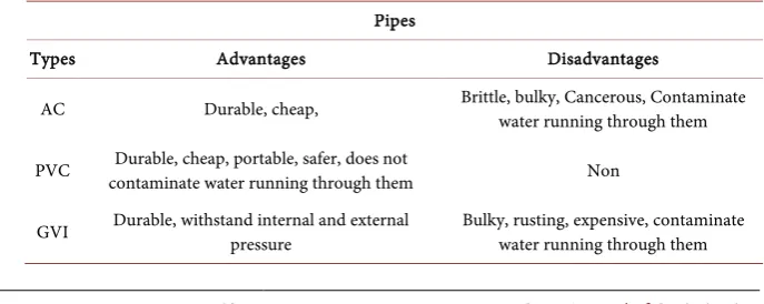
Each of the types of pipes in Table 1 has its advantages and shortcomings as presented in Table 2.

The major problems of the GVI pipes are bulkiness, rusting and expensiveness compared to the other two types. Majority of their failure result from rusting. UPVC is fast replacing GVI pipes because of their portability and durability.

Many factors are responsible for water pipe breaks. For the purpose of this paper, these factors are divided into internal and external factors, which are col-lectively called covariates. Internal factors: Internal factors include the pressure exerted by the flowing water in the pipe; the action of chemicals used in the wa-ter treatment; the diamewa-ter of the pipes and the intrinsic mawa-terial of the pipes etc. Pressure exerted by water over a long period of time on pipes leads to their break and this pressure is inversely related to the diameter of pipes. The pressure

Table 1. Types of water distribution pipes.

Pipes

Types AC UPVC GVI

Mains yes Yes yes

Branches yes Yes yes

Service (Terminals) Non Yes yes

Table 2. Water distribution pipes, advantages and disadvantages.

Pipes

Types Advantages Disadvantages

AC Durable, cheap, Brittle, bulky, Cancerous, Contaminate _{water running through them}

PVC _{contaminate water running through them} Durable, cheap, portable, safer, does not Non

DOI: 10.4236/ojop.2018.72002 43 Open Journal of Optimization is also intensified, as the pipes are located nearer to the source and reduces as the length of the pipes increases. External factors: External factors include the soil type, topography, lay-dept, shock and rust. These factors are called external be-cause they occur outside the pipes. The nature of soil in which the pipe is laid determines the rate of pipe’s break etc. The rates at which these factors occur in-fluence the maintenance decisions.

Enugu State Water Corporation Enugu

Water generation and distribution are the sole concern of the water Generation unit, Enugu State Water Corporation Enugu. The replacement and repair func-tions are the sole responsibilities of the engineering and plumbing units. The pressure under which the pumps distribute water ranges from 6 bars to 16 bars. Frequency of pipe breaks depend on the following factors namely; lay depth, to-pography, intrinsic material of the pipes, pressure, diameter of the pipes, lay lo-cation etc. Period of replacement: pipes are replaced as they break and the rule of thumb is extensively used. Maintenance actions include periodic greasing of nuts and bolts, replacement or repair of failed pipes. In most cases, the maintenances are done on demand, as there is no regularity on the time limit for the mainten-ance services. But since pipes constitute the bulk of the money cost of the water network distribution system, there is a need to develop a failure model to detect the probability of failure at any given time, the failure rate, the reliability of the pipes and the optimal replacement time of the pipes to avoid waste of water re-sources.

[1] [2] used non-homogeneous Poisson process to model the pipe failure. They were of opinion that power law process model (λ(t) = abtb−1_{) can be used to} describe the intensity of a NHPP. They define intensity as the mean number of failure, N(t), per unit time and that once the intensity has been estimated the number of failures in a given time period is Poisson.

[3][4] observed that if the parameter b is between 0 and 1, then the network is improving, but if b > 1, it shows a deteriorating network. The model parameters can be determined using either graphical or analytical analysis. We can linea-rized the mean value function M(t) by taking the logarithm of both sides to ob-tained lnM t

( )

( )

( )

ap-DOI: 10.4236/ojop.2018.72002 44 Open Journal of Optimization propriate action is to replace the equipment. [7] obtained the optimal replace-ment policy by minimizing the average annual cost of equipreplace-ment whose main-tenance cost is a function increasing with time and whose scrap value is known, and their calculations were based on average annual cost incurred on the item. They assert that the item should be replaced when the average annual cost is mi-nimal.

Water distribution pipes are repairable system because some maintenance ac-tion of repair can be done on them to restore the operaac-tion of the pipes after failures. [8] [9] [10] observed that a repairable system is a system which, after failing to perform its functions satisfactorily, can be restored to fully satisfactory performance by any method other than replacement of the entire system. Re-pairable systems shared the property that they could be repaired by replacing some failed components and returned to regular operation. Sometimes, minimal repairs bring the system reliability back to the same level it had before the fail-ure, while ‘perfect’ repairs bring the reliability back to the state of the system at the start of the operation [11] [12]. The intensity and mean value functions of a power law process PLP are λ(t; M, β) = MβtB−1 _{and V(t; M, β) = Mt}β_{; M, β > 0. β} determines how reliability decays or grows. If β < 1, the intensity function de-creases over time and the reliability improves. If β = 1, the reliability remains the same over time, but if β > 1, the reliability declines and intensity increases. Again, if β > 1, we have NHPP and for β = 1, we have HPP. λ(t) is an increasing concave (straight, convex) curve if 1 < β < 2 [13] [14] [15].

2. Overview of Poisson Process/Reliability

The Poisson Process provides a realistic model for many random phenomena. Since values of a Poisson random variable are the non-negative integers, any random phenomenon for which count of some sort is of interest is a candidate for modelling by assuming a Poisson distribution [16], thus, the first event counted by Ns(.) takes place after an exponential amount of time with parameter

DOI: 10.4236/ojop.2018.72002 45 Open Journal of Optimization production, life testing and design modifications.

Data Presentation

In this section, we present the data that is used for this work in Table 3.

3. Data Analysis

2005 - 2015 10 years

t= = ₍₁₎

18 0.9; 1,2, ,18; 1,2, ,20 20

i

x

i N

N

λ =

∑

0.9 0.09; failure per unit time 10

c c

λ

λ

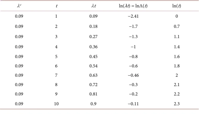
We present how the parameters of the model were determined in Table 4. The graphic method of determining the parameters of the water pipe failure model is presented in Figure 1.

(

)

lna= −2.4⇒ =a exp 2.4− =0.09

1.575

b= = ₍₅₎

Table 3. Type of pipe, Installation period, Replacement and number of Breaks.

S/No Items Values

1 Type of pipe 50 mm GVI

2 Installation period 2005

3 Period of replacement 2015

4 Length of pipe 18 ft

5 Number of pipes 20

6 Record of breaks within the period 18

7 Location Uduma Street N/Haven

Table 4. Determination of the Parameters of the Model.

λc _{t λt ln(λt) = lnΛ(t) ln(t)}

0.09 1 0.09 −2.41 0

0.09 2 0.18 −1.7 0.7

0.09 3 0.27 −1.3 1.1

0.09 4 0.36 −1 1.4

0.09 5 0.45 −0.8 1.6

0.09 6 0.54 −0.6 1.8

0.09 7 0.63 −0.46 2

0.09 8 0.72 −0.3 2.1

0.09 9 0.81 −0.2 2.2

DOI: 10.4236/ojop.2018.72002 46 Open Journal of Optimization Figure 1. Graph of lnΛ(t) versus ln(t).

Hence

( )

(

)

( )

!

n

n t

p t t n t

n

 

= − _{ } =

  

( )

(

)

0 1 exp 0.09 0.9139

p = − = (7)

( )

(

)(

)

1 1 exp 0.09 0.09 0.0823

p = − =

( )

(

) (

)

2

0.1825

2 exp 0.1825 0.0139 2!

p = − =



( )

(

) (

)

10

0.9424

10 exp 0.9424 0.000 10!

p = − = (10)

3.1. Water Pipe Failure Model

Since b > 1, then, our model assumes NHPP (λ(t)).

Equation (6) is the water pipe failure model, where p = probability; n = the number of failures; t = the time in years; a = 0.09 and b = 1.02 are the parameters of the model and a, b, t > 0.

3.2. The Reliability Function

R

(

t

)

( )

_{( )}

( )

R t t

λ

= (11)

3.3. Determination of Optimal Time of Replacement

DOI: 10.4236/ojop.2018.72002 47 Open Journal of Optimization of pipes. Reliability approach has never been used to determine the optimal wa-ter pipe replacement policy. The pipe should be replaced a little time before the reliability becomes zero. Continuous used of the pipe when the reliability be-come zero add more to the cost because the failure rate λ(t) increases rapidly as the reliability R(t) becomes zero. Hence, t (time in years) is optimal at the least reliability R(t).

4. Interpretation of Results

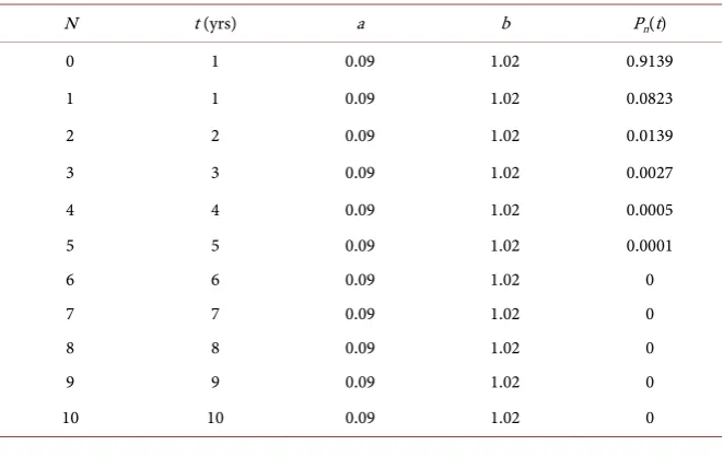
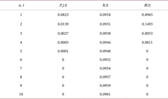
Form the data collected from Enugu State Water Corporation Enugu we obtain the parameters of our model “a” and “b” and use them to generate a table for the probability of number of failure at any given time t. Also failure rate and relia-bility of the pipes were determined and presented in Tables 4-7 respectively.

Result A:

( )

(

)

( )

!

n

n t

p t t t n

n

 

= − _{ } =

   (12)

The probability of the number of failure of pipes at a given time is presented in Table 5 below.

Result B:

( ) (

)

λ = ₍₁₃₎

The computation of the intensity function λ(t) is presented in Table 6. Table 6 shows that the intensity function, λ(t), increases with time. Result C:

( )

_{( )}

( )

R t t

λ

= ₍₁₄₎

In Table 7, we present the computation of reliability, R(t), of the water pipes.

Table 5. Probability of number of failure at Time t.

N t (yrs) a b Pn(t)

0 1 0.09 1.02 0.9139

1 1 0.09 1.02 0.0823

2 2 0.09 1.02 0.0139

3 3 0.09 1.02 0.0027

4 4 0.09 1.02 0.0005

5 5 0.09 1.02 0.0001

6 6 0.09 1.02 0

7 7 0.09 1.02 0

8 8 0.09 1.02 0

9 9 0.09 1.02 0

DOI: 10.4236/ojop.2018.72002 48 Open Journal of Optimization Table 6. Computation of the Intensity Function λ(t).

t (years) ab t0.02 _λ(t)

1 0.0918 1 0.0918

2 0.0918 1.014 0.0931

3 0.0918 1.0222 0.0938

4 0.0918 1.0281 0.0944

5 0.0918 1.0327 0.0948

6 0.0918 1.0365 0.0952

7 0.0918 1.0397 0.0954

8 0.0918 1.0425 0.0957

9 0.0918 1.0449 0.0959

10 0.0918 1.0471 0.0961

Table 7. Computation of the Reliability function R(t).

n, t Pn(t) λ(t) R(t)

1 0.0823 0.0918 0.8965

2 0.0139 0.0931 0.1493

3 0.0027 0.0938 0.0053

4 0.0005 0.0944 0.0011

5 0.0001 0.0948 0

6 0 0.0952 0

7 0 0.0954 0

8 0 0.0957 0

9 0 0.0959 0

10 0 0.0961 0

Table 7 above shows that the reliability R(t) of the pipes deteriorates with time while the failure rate of the pipes increases with time. The pipe should be replaced at the 4th _{break when the reliability of the pipes is 0.0011. Hence, it is} most reasonable to replace the pipe when the reliability is very close to zero.

5. Conclusion

DOI: 10.4236/ojop.2018.72002 49 Open Journal of Optimization

References

[1] Watson, T., Colin, C., Mason, A. and Smith, M. (2001) Maintenance of Water Distri-bution System. The 36th _{Annual Conference of American Water Works Association.}

[2] Ozger, S. and Mays, L.W. (2004) Optimal Location of Isolation Valves in Water Distribution Systems: A Reliability/Optimization Approach. Urban Water Supply Management Tools. Mcgraw-Hill, New York.

[3] Tobias, P.A. and Trindade, D.C. (1995) Applied Reliability. 2nd Edition, Chapman and Hall/CRC, New York.

[4] Gregor, V.L., Kumar, M., Ranji, R., Downey, B., Jim, V., Ken, H., Sarat, S. and Emi-ly, Z. (2006) An Adaptive Cyber Infrastructure for Threat Management in Urban Water Distribution Systems. Secure Water Resource Publications.

[5] Park, S. and Loganathan, G.V. (2000) An Optimal Replacement Scheduling for Wa-ter Distribution Systems.

[6] Jorgenson, D.W., McCall, J.J. and Rudner, R. (1967) Optimal Replacement Policy. Rand McNally and Co., Chicago.

[7] Prem, K.G and Hira, D.S. (2008) Operation Research. S. Chand & Co. Ltd, Ram Nagar, New Delhi.

[8] Lindquist, B.H. (2006). Maintenance of Repairable Systems. Journal of Statistical Planning and Inference, 136, 1701-1717.

[9] Wu, S. (2017) The Model for Failure Process of a Repairable System. The 10th interna-tional Conference on Mathematical Methods in Reliability, Goenoble, 3-6 July 2017. [10] Giogio, M., Guida, M. and Pulcini, G. (2014) Repairable System Analysis in

Pres-ence of Covariates and Random Effects. Elsevier, 131, 271-281.

[11] Masini, L., Antonio, P., Ruggeri, F. and Emmanuela, S. (2006) On Bayesian Models Incorporating Covariates in Reliability Analysis of Repairable Systems. Applied Sta-tistics Models in Business and Industry, 20, 253-264.

[12] Karol, A. (2015) Stochastic Modeling of the Repairable System. Journal of KONBiN, 3, 5-14.

[13] Ruggeri, F. and Siva, S. (2005) On Modelling Change Points in Non-Homogeneous Poisson Process. Statistical Inference for Stochastic Processes, 8, 311-329.

[14] Argiento, R., Pievatolo, A., Ruggeri, F., Cagno, E. and Macini, M. (2003) Seasonal Pattern and Double Measurement Scale in Modelling Failures in Underground Trains. 3rd International Conference on Mathematical Methods in Reliability. [15] Guo, R., Ascher, H. and Love, E. (2001) Towards Practical and Synthetical

Model-ling of Repairable Systems. Economic Quality Control, 16, 147-182.

https://doi.org/10.1515/EQC.2001.147

[16] Graybill, F.A., Boes, D.C. and Mood, A.M. (1974) Introduction to the Theory of Statistics. McGraw-Hill Book Company, New York.

[17] Chat Field, C. and Zidek, J.V. (1995) Modelling and Analysis of Stochastic Systems. Chapman and Hall, London.

[18] Barlow, R.E. and Proschan, F. (1975) Statistical Theory of Reliability and Life Test-ing Probability Models. Holt, Rinehart and Winston, Inc., Boston.

[19] Smith, R.L. (1991) Statistical Analysis of Reliability Data. Chapman and Hall, London. [20] Irwin, M. and John, E.F. (1987) Probability and Statistics for Engineers. 3rd Edition,