Water Tank Fish Algorithm: A New Metaheuristic for Optimization

Water-Tank Fish Algorithm: A New Metaheuristic for

Optimization

Madhup Sukoon

Haider Banka, PhD

ABSTRACT

This paper aims to introduce a new metaheuristic : The Water-Tank Fish Algorithm, modeled after the workings of the swim bladder in fish, to non-deterministically compute the optima for numerical op-timization problems. To balance the explorative-exploitative behav-ior of a search, the proposed method uses a search localization rou-tine which, after a general exploration, restricts the search to cer-tain areas of the graph and intensifies it as the algorithm advances. The proposed method is tested over 40 benchmark mathemati-cal functions and the results were found to be very encouraging.

General Terms

Metaheuristic, Nature Inspired, Optimization

Keywords

Fish, Buoyancy, Metaheuristic, Nature Inspired, Optimization

1. INTRODUCTION

The conventional approach to solving problems by computers is often found to be inadequate when solving real life problems, be it due to the multimodality of the problem, non-flexible construc-tion or due to the sheer vastness of the search space. Such con-ditions render the conventional extensive search algorithms use-less as the cost of finding the solution(s) in terms of CPU cycles and time, using such algorithms is very high. On the other hand, when similar problems are encountered in nature, the nature uses novel algorithms that are a result of several millennia of evolu-tion. The algorithms used by nature are usually very efficient and outperform the algorithms designed by humans in terms of effi-ciency, accuracy and reliability. The algorithms used by nature are usually comprised of small agents that individually execute a very small and simple part of the algorithm, but when the output of each such agent is combined, the resulting output is often observed to be prominent. Natural algorithms are usually simple implementa-tions of physical, chemical or mathematical rules and laws in nature and Nature Inspired Metaheuristics is a relatively new paradigm of Computer Science that aims at understanding and modeling such algorithms to create faster and more efficient ways for computers to solve real life problems. This paper presents a nature inspired al-gorithm, called the Water-Tank Fish Algorithm that simplifies and speeds up the task of optimizing mathematical functions. This algo-rithm is inspired from the working of the swim bladder in various marine animals. The swim bladder is an organ found in most of

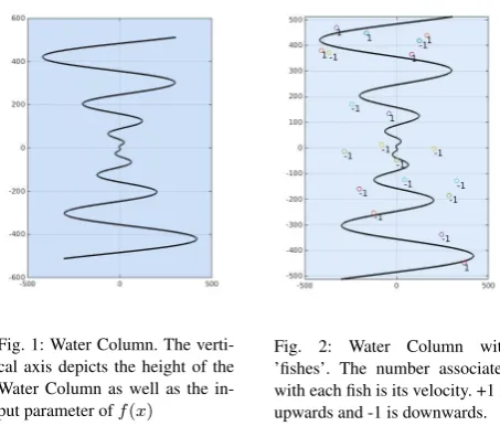
Fig. 1: Water Column. The verti-cal axis depicts the height of the Water Column as well as the in-put parameter off(x)

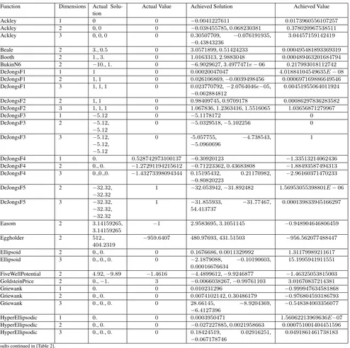
Fig. 2: Water Column with ’fishes’. The number associated with each fish is its velocity. +1 is upwards and -1 is downwards.

the aquatic animals which allows them to change their altitude in water without much effort. The swim bladder is a basically a hol-low pouch that contains air and alhol-lows the animal to change its size by contracting muscles, thus changing the density of its own body. Whenever there is a need for the animal to rise towards the surface, the swim bladder is allowed to expand, hence greatly reducing the density of the animal. Now, the buoyancy force acting on it pushes the animal upwards and the animal is able to change its altitude and go towards the surface with no or very little effort. Similarly, whenever there is a need for the animal to descend towards the base of the water body, the swim bladder is contracted, hence increasing the density of the animal’s body and allowing gravity to bring it closer to the base of the water body with no or very less effort.

2. WORKING

For the sake of simplicity, the Schwefel’s Function in 1 Dimension was considered as the function to be minimized. Thus, the fitness functionf(x)becomes:

f(x) =−x·sin(p|x|)

heights[Figure 2], each fish having a unit mass. The ’Fishes’ are intelligent because like real life fishes, they can change the up-ward(buoyant)/downward(weight) forces acting on them by chang-ing their volume and thus attain an altitude of their choice in the water column. Each fish is given a unit velocity but the direction of the velocity(upwards or downwards) is randomized.

From here on, the algorithm runs independently. Each fish obtains its fitness value by evaluatingf(x) at its current height. Fitness value for each fish is calculated and the minimum and the maxi-mum fitness values for each iteration are found out. Next, based on its own fitness value, the least and the greatest fitness values of the previous iteration and its current velocity, each fish changes its volume to a new value which gives the fish a new velocity. The algorithm is designed in such a way that whenever the fish goes from a better solution to a worse solution, its velocity increases. Also, whenever the fish approaches a good solution, its velocity decreases. This feature gives the algorithm a good control over the Eplorative-Exploitative behaviour. After attaining a new velocity, each fish travels with the new velocity for a fixed amount of time 0

T ransT ime0(Translatoray Time) which is a tunable parameter.

3. THEORY AND DERIVATIONS

We know that the weight, or the downward force (Fw) and the

buoyant, or the upward force (Fb)acting on an object of massm

and volumevimmersed in a liquid of densityρare Fw=m·g

Fb=v·ρ·g

wheregis the gravitational acceleration. The net force acting on such an object would be the resultant of the gravitational and the buoyant forces. Since the two forces act in opposite directions, the resultant can be calculated by subtracting them.

F =Fb−Fw

The net force on an object can also be denoted as the product of its massmand its accelerationa. Therefore,

m·a=v·ρ·g−m·g

For an object of unit mass submerged in a fluid of unit density, the equation becomes

a= (v−1)·g

Assuming this object was subjected to this acceleration for time tand multiplying both sides byt, the following equation comes forth:

a·t= (v−1)·g·t

N ewV elocity=CurrentV elocity+a·t

Using this equation in the context of the algorithm, for each fish of unit mass in a column of water of unit density, the following equation can be used to update the velocity of the fish.

N ewV elocity=CurrentV elocity+ (v−1)·g·t

The termg·tis dimensionally equal to velocity.gis a constant, and the algorithm is constructed to adjust the value oftsuch that g·tbecomes equal to the current velocity of the object.

Hence,

N ewV elocity=CurrentV elocity+(v−1)·CurrentV elocity

⇒N ewV elocity=CurrentV elocity·v

The volume of the fish is an indicator of the fitness of the solu-tion being represented by the current locasolu-tion of the fish. The fish should slow down as it approaches a good solution to enable the exploitation of that solution. Also, the velocity of a fish should in-crease when it approaches a bad solution so that it can be skipped quickly. Therefore, a relation between the fitness of a fish’s loca-tion and the volume of that fish is established in such a way that in a given iteration, the fittest fish will have a volume of0and the most unfit fish will have a volume of1. This can be further scaled by multiplying it with any scalar valuexwhich will multiply the velocity of the least fit fish byxand set the velocity of the fittest fish as0while scaling the velocity of all other fishes in this range. To do this, the volumevof a fishjin the iterationiis defined as:

vji=x·

maxf iti−F itnessF unction(P ositionj)

maxf iti−minf iti

and arrive at the equation to update the velocity of a given fishjin a given iterationi:

Vji=Uji·x·

maxf iti−F itnessF unction(P ositionj)

maxf iti−minf iti

wherexis the scaling factor,VjiandUjiare respectively the new

and current velocities of the fishjandmaxf itiandminf itiare

the outputs of the fitness function of the fittest and the least fit fish respectively for a given iterationi.

4. ALGORITHM AND PARAMETERS

Following are the components and parameters that build up the al-gorithm:

n is the number of fishes/candidates used per dimension, e.g. using a value ofn = 25would cause the algorithm to run with 50 candidates when evaluating a function in two dimensions. FitnessFunction() is the function that returns the relative fitness,

or goodness of a solution for the function to be optimized. For example, in case of finding the maxima of a function, the fit-ness function would be the same as the function to be optimized, whereas to find the minima of a function, the fitness function would be the reciprocal of the function to be optimized. position of a candidate refers to the solution being represented by

that candidate.

k is a tunable parameter that determines the minimum non zero ve-locity at which a fish can travel. Smaller the value ofk, greater is the search intensity in the exploitative phase. However, very small values ofkwill slow down the convergence of the algo-rithm. Good results were obtained fork←0.1

TransTime corresponds to the Step Size for the algorithm. Very small values will slow down the convergence whereas large val-ues may result in optimas getting skipped.

Dmax, Dmin are respectively the maximum and minimum

val-ues allowed for a given dimension. Any candidate going beyond these values is reset to a valid position.

x is the scaling factor which determines by how many times the velocity of each candidate increases or decreases. For example, setting the value of 2 would cause the velocity of the least fit candidate to double.

Initialization:: Create a set of N randomly selected candidates (fishes) and assign each one a unit velocityV in a random direction.

foreachj∈Ndo

F itnessj←F itnessF unction(P ositionj)

end

foreachiteration ido

maxf iti←max(F itness1, F itness2...F itnessN)

minf iti←min(F itness1, F itness2...F itnessN)

foreachj∈Ndo

Vj←Vj·x·

maxf iti−F itnessF unction(P ositionj)

maxf iti−minf iti

if(Vj6= 0)and(|Vj|< k)then

Vj←k·Vˆj

end

foreachdimension Ddo

P ositionjD←P ositionjD+VjD·T ransT ime

if(P ositionjD > Dmax)or(P ositionjD < Dmin)

then

P ositionjD ←Random(Dmax, Dmin)

end end

F itnessj←F itnessF unction(P ositionj)

end

ifmaxf iti< max(F itness1, F itness2...F itnessN)then

foreachj∈Ndo

ifF itnessj==maxf itithen

Vj←k·RandomV elocityˆ

end end end end

Algorithm 1:The Water-Tank Fish Algorithm

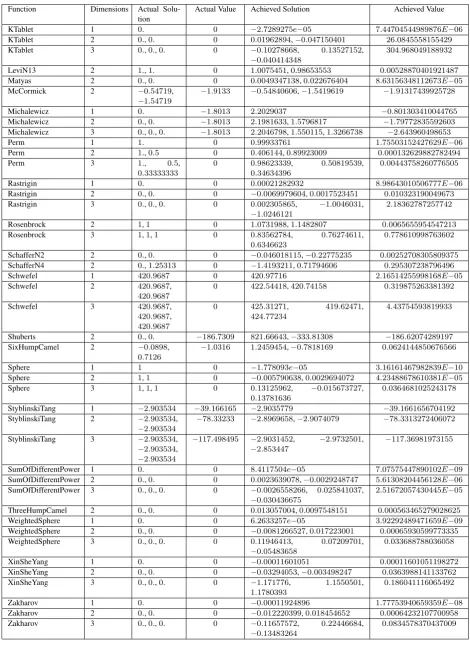
5. REUSLT AND CONCLUSION

The Algorithm was found to be working well for over 30 tested benchmark functions and the results were found quite encourag-ing. The results for these tests using the general hyperparameters n= 25, x= 10, T ransT ime = 1, k = 0.5and 1000 iterations are present in [Table 1]. The selected hyperparameters resulted in quick convergence of few functions, while non-convergence of some others. Further research into enhancement of the algorithm and improving the parameters may result in faster and better con-vergence for optimization problems.

6. REFERENCES

[1] Berat Do˘gan and Tamer ¨Olmez. A new metaheuristic for nu-merical function optimization: Vortex search algorithm. Infor-mation Sciences, 293:125–145, 2015.

[2] James Kennedy. Particle swarm optimization. InEncyclopedia of machine learning, pages 760–766. Springer, 2011.

[3] Esmat Rashedi, Hossein Nezamabadi-Pour, and Saeid Saryazdi. Gsa: a gravitational search algorithm. Information sciences, 179(13):2232–2248, 2009.

[4] S Salcedo-Sanz, J Del Ser, I Landa-Torres, S Gil-L´opez, and JA Portilla-Figueras. The coral reefs optimization algorithm: a novel metaheuristic for efficiently solving optimization prob-lems.The Scientific World Journal, 2014, 2014.

[5] Sait Ali Uymaz, Gulay Tezel, and Esra Yel. Artificial algae al-gorithm (aaa) for nonlinear global optimization.Applied Soft Computing, 31:153–171, 2015.

Table 1. : 1000 Iterations of the algorithm with the hyperparametersn= 25, x= 10, T ransT ime= 1, k= 0.5

Function Dimensions Actual

Solu-tion

Actual Value Achieved Solution Achieved Value

Ackley 1 0 0 −0.0041227611 0.0173960556107257

Ackley 2 0,0 0 −0.038455785,0.068230381 0.378020967538511

Ackley 3 0,0,0 0 0.30507709, −0.076191935,

−0.43843236

3.04457159142419

Beale 2 3.,0.5 0 3.0571899,0.51424233 0.000495481893369319

Booth 2 1.,3. 0 1.0163313,2.9883048 0.000489463201684794

BukinN6 2 −10.,1. 0 −6.9029627,3.4977471e−06 0.217993018112742

DeJongsF1 1 1 0 0.00020047047 4.01884104549635E−08

DeJongsF1 2 1,1 0 0.026106869,−0.0039498456 0.000697169886649546

DeJongsF1 3 1,1,1 0 0.023770792, −2.0764046e−05,

−0.062884812

0.00451955064011924

DeJongsF2 2 1,1 0 0.98409745,0.9709178 0.00086297836283582

DeJongsF2 3 1,1,1 0 1.067836,1.2363416,1.5516065 1.03656871279967

DeJongsF3 1 −5.12 0 −5.1178172 0

DeJongsF3 2 −5.12,

−5.12

0 −5.0329518,−5.102256 0

DeJongsF3 3 −5.12,

−5.12,

−5.12

0 -5.057755, −4.738543,

−5.0960696

1

DeJongsF4 1 0. 0.528742973100137 −0.30920123 −1.33513214062436

DeJongsF4 2 0.,0. −1.27291194215612 −0.71223362,0.43683808 −1.88493587494313

DeJongsF4 3 0.,0.,0. −1.43273398094344 0.15195432, 0.21170982,

−0.80820223

−2.96160371470233

DeJongsF5 2 −32.32,

−32.32

1 −32.053942,−31.892482 1.56953055398801E−06

DeJongsF5 3 −32.32,

−32.32,

−32.32

1 −31.855933, −31.77467,

54.413737

0.000139833945166297

Easom 2 3.14159265,

3.14159265

−1 2.9583695,3.1051145 −0.948904646806459

Eggholder 2 512.,

404.2319

−959.6407 480.97693,431.51503 −956.562077488447

Ellipsoid 2 0.,0. 0 0.1676686,0.0011329992 1.31179989211617

Ellipsoid 3 0.,0.,0. 0 −2.1879088, −0.10190603,

0.00016676634

15.1995941911551

FiveWellPotential 2 4.92,−9.89 −1.4616 −4.4899612,−9.9246877 −1.46325053815003

GoldsteinPrice 2 0.,−1. 3 −0.0066038267,−0.99761103 3.01670837214381

Griewank 1 0. 0 0.010231296 −0.999947634581868

Griewank 2 0.,0. 0 0.0074102142,0.30486179 −0.976804593186793

Griewank 3 0.,0.,0. 0 28.66145, −8.9204369,

−6.4127396

−0.548384003356077

HyperEllipsodic 1 0. 0 0.0003950471 1.56062213969636E−07

HyperEllipsodic 2 0.,0. 0 −0.027227885,0.0021958663 0.000751001404451596

HyperEllipsodic 3 0.,0.,0. 0 0.18424519, 0.02916251,

−0.067178746

0.0491861461738183

Table 2. : Contd.: 1000 Iterations of the algorithm with the hyperparametersn= 25, x= 10, T ransT ime= 1, k= 0.5

Function Dimensions Actual

Solu-tion

Actual Value Achieved Solution Achieved Value

KTablet 1 0. 0 −2.7289275e−05 7.44704544989876E−06

KTablet 2 0.,0. 0 0.01962894,−0.047150401 26.0845558155429

KTablet 3 0.,0.,0. 0 −0.10278668, 0.13527152,

−0.040414348

304.968049188932

LeviN13 2 1.,1. 0 1.0075451,0.98653553 0.00528870401921487

Matyas 2 0.,0. 0 0.0049347138,0.022676404 8.63156348112673E−05

McCormick 2 −0.54719,

−1.54719

−1.9133 −0.54840606,−1.5419619 −1.91317439925728

Michalewicz 1 0. −1.8013 2.2029037 −0.801303410044765

Michalewicz 2 0.,0. −1.8013 2.1981633,1.5796817 −1.79772835592603

Michalewicz 3 0.,0.,0. −1.8013 2.2046798,1.550115,1.3266738 −2.643960498653

Perm 1 1. 0 0.99933761 1.75503152427629E−06

Perm 2 1.,0.5 0 0.406144,0.89923009 0.000132629882782494

Perm 3 1., 0.5,

0.33333333

0 0.98623339, 0.50819539,

0.34634396

0.00443758260776505

Rastrigin 1 0. 0 0.00021282932 8.98643010506777E−06

Rastrigin 2 0.,0. 0 −0.0069979604,0.0017523451 0.010323190049673

Rastrigin 3 0.,0.,0. 0 0.002305865, −1.0046031,

−1.0246121

2.18362787257742

Rosenbrock 2 1,1 0 1.0731988,1.1482807 0.0065655954547213

Rosenbrock 3 1,1,1 0 0.83562784, 0.76274611,

0.6346623

0.778610998763602

SchafferN2 2 0.,0. 0 −0.046018115,−0.22775235 0.00252708305809375

SchafferN4 2 0.,1.25313 0 −1.4193211,0.71794606 0.295307238796496

Schwefel 1 420.9687 0 420.97716 2.16514255998168E−05

Schwefel 2 420.9687,

420.9687

0 422.54418,420.74158 0.319875263381392

Schwefel 3 420.9687,

420.9687,

420.9687

0 425.31271, 419.62471,

424.77234

4.43754593819933

Shuberts 2 0.,0. −186.7309 821.66643,−333.81308 −186.62074289197

SixHumpCamel 2 −0.0898,

0.7126

−1.0316 1.2459454,−0.7818169 0.0624144850676566

Sphere 1 1 0 −1.778093e−05 3.16161467982839E−10

Sphere 2 1,1 0 −0.005790638,0.0029694072 4.23488678610381E−05

Sphere 3 1,1,1 0 0.13125962, −0.015673727,

0.13781636

0.0364681025243178

StyblinskiTang 1 −2.903534 −39.166165 −2.9035779 −39.1661656704192

StyblinskiTang 2 −2.903534,

−2.903534

−78.33233 −2.8969658,−2.9074079 −78.3313272406072

StyblinskiTang 3 −2.903534,

−2.903534,

−2.903534

−117.498495 −2.9031452, −2.9732501,

−2.853447

−117.36981973155

SumOfDifferentPower 1 0. 0 8.4117504e−05 7.07575447890102E−09

SumOfDifferentPower 2 0.,0. 0 0.0023639078,−0.0029248747 5.61308204456128E−06

SumOfDifferentPower 3 0.,0.,0. 0 −0.0026558266, 0.025841037,

−0.030436675

2.51672057430445E−05

ThreeHumpCamel 2 0.,0. 0 0.013057004,0.0097548151 0.000563465279028625

WeightedSphere 1 0. 0 6.2633257e−05 3.92292489471659E−09

WeightedSphere 2 0.,0. 0 −0.0081266527,0.017223001 0.00065930599773335

WeightedSphere 3 0.,0.,0. 0 0.11946413, 0.07209701,

−0.05483658

0.033688788036058

XinSheYang 1 0. 0 −0.00011601051 0.00011601051198272

XinSheYang 2 0.,0. 0 −0.03294053,−0.003498247 0.0363988141133762

XinSheYang 3 0.,0.,0. 0 −1.171776, 1.1550501,

1.1780393

0.186041116065492

Zakharov 1 0. 0 −0.00011924896 1.77753940659359E−08

Zakharov 2 0.,0. 0 −0.012220399,0.018454652 0.00064232107700958