Improving the Classification accuracy of Noisy Dataset by Effective Data Preprocessing

Improving the Classification accuracy of Noisy Dataset

by Effective Data Preprocessing

K. V. Uma

Department of Information Technology

Thiagarajar College of Engineering

ABSTRACT

Decision tree is a technique commonly used in data mining. Issues in decision tree algorithms are working with continuous attributes and missing values, avoiding over fitting, super attributes. Handling noisy data is the challenging factor in data mining research. Noisy data is meaningless data. It unnecessarily increases the amount of storage space required and can also adversely affect the results of any data mining analysis. Predicting the result from such noisy data is the complicated factor. The commonly used algorithm for classification problems are decision stump, ensemble models, SVM, and decision tree algorithms. The performance of the algorithm resulted in lower accuracy when comparing with the noiseless data result. Thus in this paper, data is collected and noise is added to the data, and then it is preprocessed for handling missing values. The preprocessed data is then provided as the input for the feature selection technique. Most relevant features are selected using correlation based subset feature selection technique. The selected features are provided as the input of Credal C4.5 algorithm and decision tree is constructed. The result is analyzed with various data with (5,10,20,30)% noise level. This technique improves the performance of the algorithm with (1-5)% improvement in accuracy compared to the existing result.

Keywords

Classification, Noisy Data , Feature Selection, Data Preprocessing.

1.

INTRODUCTION

Real-world data, which is the input of the Data Mining algorithms, are affected by several components; among them, the presence of noise is a key factor Noise is an unavoidable problem, which affects the data collection and data preparation processes in Data Mining applications, where errors commonly occur. Noise has two main sources implicit errors introduced by measurement tools, such as different types of sensors; and random errors introduced by batch processes or experts when the data are gathered, such as in a document digitalization process. Classification problems containing noise are complex problems and accurate solutions are often difficult to achieve. The presence of noise in the data may affect the intrinsic characteristics of a classification problem since these corruptions could introduce new properties in the problem domain. For example, noise can lead to the creation of small clusters of examples of a particular class in areas of the domain corresponding to another class, or it can cause the disappearance of examples located in key areas within a specific class. The boundaries of the classes and the overlapping between them are also factors that can be affected as a consequence of noise. All these alterations difficult the knowledge extraction from the data and spoil the models obtained using that noisy data when they are compared to the models learned from clean data, which represent the real implicit knowledge of the problem.

Therefore, data gathered from real-world problems are never perfect and often suffer from corruptions that may hinder the performance of the system in terms of the classification accuracy, model building time, size and interpretability of the classifier. Predicting the result from such noisy data is the complicated factor. The commonly used algorithm for classification problems is decision stump, ensemble models (bagging and Adaboost and random forest), SVM, and decision tree algorithms. The performance of the algorithm resulted in lower accuracy when comparing with the noiseless data result.

2.

RELATED WORK

comparing to the classic C4.5 algorithm in the presence of domains of class noise.[2][9] The application of artificial intelligence approaches to credit risk assessment has meant a development over classic systems in the former years. Trivial developments in the schemes about insolvency and credit scoring forecast can presume great profits. Then, any improvement represents a high interest to banks and financial institutions. Current mechanisms demonstrate that the better results for this kind of tasks are achieved by ensembles of classifiers. A very simple base classifier which is imprecise probabilities and uncertainty measures based achieves an improved trade-off amongst certain features of interest is addressed in this paper. The dataset used in this experiment is Australian, German, Iranian, Japanese, Polish, and UCSD. The advantage of the experimental results present that for credit scoring and insolvency prediction this simple classifier is a motivating choice to be used as a base classifier in ensembles, in addition, it proves that the individual recital of a classifier is the key point to be designated for an ensemble system.[3] A key topic in machine learning is the structure of well-organized and actual decision trees ruins because of their easiness and litheness. To build immediate optimum decision trees a lot of empirical algorithms have been proposed to overcome the problem. Most of them, nevertheless, are greedy algorithms in which the drawback is only local optimums are obtained. In addition, predictable split criteria they used are based on one-term which lacks adaptableness to diverse datasets. A Tsallis Entropy Information Metric (TEIM) algorithm is proposed to address this problem. The dataset used for experiment are Hayes, Wine, Glass, Harberman, Monks, Scale, Vehicle, Cmc, Yeast, Car, Image, Chess, EEG, Letter. The TEIM algorithm takes advantages of the generalization ability of two- term Tsallis entropy and the low greediness property of two-stage approach. In experimental results comparison of state-of-the-art decision trees algorithms with the TEIM algorithm in which it produces statistically improved decision trees and in addition robust to noise.[4] A number of problems that are experienced when handling biological data for classification are over-fitting, noisy instances, class-imbalance data and etc. A new adaptive rule-based classifier for multi-class classification of biological data is proposed for solving the problems. The dataset used in the experiment is Appendicitis, Breast-cancer, Contraceptive, Ecoli, Heart, Pima-diabetes, Iris, Soybean, Thyroid, Yeast. The proposed rule-based classifier combines the random subspace and boosting approaches with an ensemble of decision trees to construct a set of classification rules without involving global optimization. The classifier considers random subspace approach to avoid overfitting, boosting approach for classifying noisy instances and ensemble of decision trees to deal with a class-imbalance problem. The performance of proposed classifier is tested and compared to well-approved existing machine learning and data mining algorithms. The experimental results indicate that the proposed classifier has exemplary classification accuracy on different types of biological data with noisy and misclassified variants are optimized to increase test performance.[5] To diminish the network convolution, a pruning proposal by using Q-values is applied to reduce the number of prototypes generated by QFAM. A two-stage hybrid model for data classification and rule extraction is proposed in this paper. The first stage uses a Fuzzy ARTMAP (FAM) classifier with Q-learning (known as QFAM) for incremental learning of data samples, while the second stage uses a Genetic Algorithm (GA) for rule extraction from QFAM. The dataset used in the experiment are Iris, PID, Dermatology, Glass,Sonar, Wine, Statlog (Heart). Given a new data sample,

the resulting hybrid model, known as QFAM-GA, is able to provide prediction pertaining to the target class of the data sample as well as to give a fuzzy if-then rule to explain the prediction. The main significance of this research is a usable and useful intelligent model (i.e., QFAM-GA) for data classification in noisy conditions with the capability of yielding a set of explanatory rules with minimum antecedents. In addition, QFAM-GA is able to maximize accuracy and minimize model complexity simultaneously. The empirical outcome positively demonstrates the potential impact of QFAM-GA in the practical environment, i.e., providing an accurate prediction with a concise justification pertaining to the prediction to the domain users, therefore allowing domain users to adopt QFAM-GA as a useful decision support tool in assisting their decision-making processes.[6] Building intellectual classification replicas can basically assist in diagnosis and medical data analysis in particular while the existing medical databases are illustrated as noisy data. On a number of noisy medical data, a variety of decision tree classifiers based on supervised machine learning technique is addressed in this paper. These tree based algorithms are categorized into three, first is the ensemble models such as bagging, Adaboost, and random forest, next is single tree classifiers such as Decision Stump, C4.5, and Rep Tree, and the last is Credal Decision Trees (CDTs), which is uncertainty measures and imprecise probabilities based. The dataset used in this experiment is Thrombosis Disease, Hypothyroid Disease, Arrhythmia Disease, Heart Disease. Advantage on the investigation of the technique; it is identified as the ensemble classifiers described higher classification accuracy than single tree classifiers approaches. In addition, the CDTs smash the single tree classifiers and evidenced approximately the same classification accuracy as ensemble models in which building time of the replica is smaller. It is especially appropriate in noisy domains of numerical attributes databases.[7]

Segment, Sick, Solar-flare2, Sonar, Soybean, Spambase, Spectrometer, Splice, Sponge, Tae, Vehicle, Vote, Vowel, Waveform, Wine, Zoo. In the new procedure of a special type of CDT is addressed in terms of the split criterion used is explained in this paper which is termed as Credal-C4.5. This criterion is more robust to noise in comparison and the CDTs depend on a parameter 's'which is directly related to the size of the built tree. An experimental research is carried out for diverse values of s and that are compared with distinct label noise levels when the data sets are classified. Experimental results are concluded and evidenced as the choice of the correct value for s is a key point if it is possible to estimate the noise level of a data set, in order to obtain notably better results.[9] Handling the effect of noisy data on the performance of classifier learning algorithms is necessary to improve their reliability and has motivated the study of how to generate and introduce noise into the data. Noise generation can be characterized by three main characteristics:

 The place where the noise is introduced. Noise may affect the input attributes or the output class, impairing the learning process and the resulting model;

 The noise distribution. The way in which the noise is present can be, for example, uniform or Gaussian;

 The magnitude of generated noise values. The extent to which the noise affects the dataset can be relative to each data value of each attribute, or relative to the minimum, maximum and standard deviation for each attribute.

In real-world datasets the initial amount and type of noise present are unknown. Therefore, no assumptions about the base noise type and level can be made. For this reason, these datasets are considered to be noise free, in the sense that no recognizable noise has been induced into them. In order to control the amount of noise in each dataset and check how it affects the classifiers, noise is introduced into each dataset in a supervised manner in this study. Noise is added to the class label of the dataset

3.

METHODOLOGY

The flow of the method described is as shown in figure 1, in which the datasets are collected. Then preprocessing step is processed and features are extracted using feature selection technique. The extracted features are processed using a Credal C4.5 algorithm and then the results are compared and analyzed. Modules that are carried out to meet the objectives are as follows;

• Data collection

• Data Preprocessing

• Feature Selection

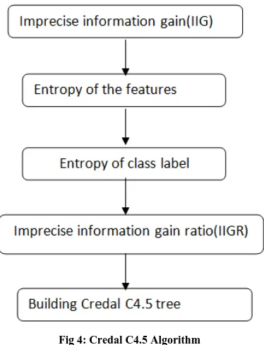
• Credal C4.5 algorithm

◦ Imprecise information gain(IIG) ◦ Entropy of the features

◦ Entropy of class label

◦ Imprecise information gain ratio(IIGR) ◦ Building Credal C4.5 tree

[image:3.595.332.560.74.180.2]

• Comparison and Analyzing the result

Fig 1. Architecture diagram

3.1

Data Preprocessing

In this step, dataset is collected and the missing values are analyzed as shown in figure 2. If there is blank space in the dataset it is replaced and noise is added to the dataset. The obtained result is the preprocessed data.

Fig2. Data preprocessing

3.2

Feature Selection

The preprocessed data is processed for feature extraction which is described in figure 3. For feature selection, CfsSubsetEval technique is used and in which most relevant attributes are selected using the best first method. The irrelevant attributes are removed and most influencing factors are identified.

Fig. 3 Feature Selection Process

3.3

Credal C4.5 Algorithm

A decision tree is one of the methods in predictive analysis. For handling noisy data Credal C4.5 algorithm is used, The steps that are involved in Credal C4.5 algorithm are Imprecise information gain(IIG), Entropy of the features, Entropy of class label, Imprecise information gain ratio(IIGR) calculation and based on the gain ratio decision tree is constructed and with this confusion matrix is formed through which accuracy is calculated. Using the eqn 1, Imprecise Information Gain(IIG) is calculated for all attributes with respect to the class label. It is defined as the difference between the entropy of the class label with the summation of the probability function of all variables and entropy of the variables with respect to class label.

IIG C, X = H∗ _{K C − P X = x} i ∗ i

H ∗ _{K C X = x}

i (1)

[image:3.595.324.536.430.544.2]

[image:4.595.330.542.75.182.2]

Fig 4: Credal C4.5 Algorithm

Equation 2 is used for calculating the entropy value of all attributes. It is defined as the summation of probability all attributes.

𝐻 𝑋 = − 𝑃𝑖𝑙𝑜𝑔2𝑃𝑖 (2)

Pi =probability of number of occurrence of the features

Equation 3 is used for calculating the entropy value of the class label. It is defined as the ratio of a frequency of the set of values plus 1 to the number of instances plus s parameter.

H∗ _{K C = −}nc+1

N+s (3)

N=Number of instances

nc=Frequency of the set of values

IIGR =IIG (C,X)_H(X) (4)

Using the above Equation 4 ,a IIGR is calculated in which it is defined as the ratio of Imprecise Information Gain and entropy of the features. Based on the IIGR value calculated credal C4.5 algorithm’s decision tree is constructed. Using this tree confusion matrix is formed and then accuracy is calculated.

Algorithm for Building Credal C4.5 Tree

Pseudo code to build credal-c4.5 algorithm tree;



Input: Dataset S



Tree={}



if S is satisfied or any stopping criteria met then

o

terminate



end if



for all attribute n € S do

o

compute Imprecise Information theoretic criteria if we split on n



end for

o

𝑛

_{𝑏𝑒𝑠𝑡}=Best attribute with respect to the above-computed value

o

Tree =Create a decision node in which

𝑛

_{𝑏𝑒𝑠𝑡} as the root node

o

𝑆

_𝑖= Induced sub-dataset from S based on

𝑛

_{𝑏𝑒𝑠𝑡}



for all

𝑆

_𝑖do

o

Treei =CredalC4.5(

𝑆

𝑖)

o

Attach

𝑇𝑟𝑒𝑒

_𝑖 to the corresponding branch of Tree



end for



return Tree

4.

RESULTS AND DISCUSSIONS

[image:4.595.75.262.77.321.2]

that are individually highly correlated with the class but have low inter-correlation. The subset evaluators use a numeric measure, such as conditional entropy, to guide the search iteratively and add features that have the highest correlation with the class. CFS evaluates the worth of a subset of attributes by considering the individual predictive ability of each feature along with the degree of redundancy between them. Correlation coefficients are used to estimate the correlation between a subset of attributes and class, as well as inter-correlations between the features. The relevance of a group of features grows with the correlation between features and classes and decreases with growing inter-correlation. CFS is used to determine the best feature subset and is usually combined with search strategies such as forward selection, backward elimination, bi-directional search, best-first search and genetic search. The equation for CFS is given in equation 4 as

𝑟

_𝑧𝑐

=

𝑘𝑟 𝑧𝑖 𝑘+𝑘(𝑘−1)𝑟 𝑖𝑖

(4)

Where

𝑟

_𝑧𝑐the correlation between the summed feature subsets and the class is variable,

𝑘

is the number of subset features,

𝑟

_𝑧𝑖 is the average of the correlations between the subset features and the class variable,

𝑟

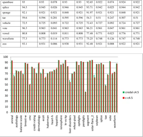
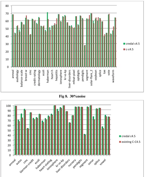
_𝑖𝑖 is the average inter-correlation between subset features. The Credal C4.5 algorithm is used for handling the noisy data and to minimize the size of the tree to get better performance result. The Credal C4.5 algorithm is implemented using the Weka package and the necessary changes are done in the J48 algorithm which is the classic C4.5 algorithm. The split criteria of the Credal C4.5 algorithm are the imprecise information gain ratio. IIGR is defined as the ratio of imprecise information gain to the entropy of the features or attributes. With this tree is generated and compared with the dataset the measures such as TPrate, FPrate, Precision, Recall, F-measure are calculated. The accuracy is calculated for these

dataset Anneal, Arrhythmia, Audiology, Autos, Balance-scale, Breast-cancer, Wisconsin-breast-cancer, Car, Cmc, Horse-colic, Credit-rating, German-credit, Dermatology, Pima-diabetes, Ecoli, Glass, Haberman, Cleveland-14-heart-disease, Hungarian-14-heart-Cleveland-14-heart-disease, Heart-statlog, Hepatitis, Hypothyroid, Ionosphere, Iris, kr-vs-kp, Letter, Liver-disorders, Lymphography, Mfeat-pixel, Nursery, Optdigits, Page-blocks, Pendigits, Primary-tumor, Segment, Sick, Solar-flare2, Sonar, Soybean, Spambase, Spectrometer, Splice, Sponge, Tae, Vehicle, Vote, Vowel, Waveform, Wine, Zoo with 5%,10%,20%,30% and 0%noise level. This accuracy is compared with the existing c-c4.5 algorithm as shown in figure 5,6,7, 8 and 9 respectively. The obtained result is tested using Wilcoxon signed rank test and Friedman test.The Wilcoxon signed rank test is a non-parametric test. When the word non-parametric is used in stats, it doesn’t quite mean that you know nothing about the population. It usually means that you know the population data does not have a normal distribution. The Wilcoxon signed rank test should be used if the differences between pairs of data are non-normally distributed. The steps that are carried out in this test are;

 Subtract B from treatment A to get the differences

 Place the differences in order and then rank them. Ignore the sign when placing in rank order.

 Make a third column and note the sign of the difference.

 Calculate the sum of the ranks of the negative differences,not the actual differences (W–).

 Calculate the sum of the ranks of the positive differences (W+).

[image:5.595.83.518.477.770.2]

 Then Z-score is calculated by which p-value is computed.

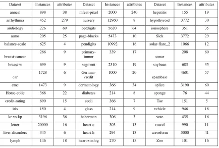
Table 1 – Instances and number of attributes of the dataset

Dataset Instances attributes Dataset Instances attributes Dataset Instances attributes

anneal 898 38 mfeat-pixel 2000 240 hepatitis 155 19

arrhythmia 452 279 nursery 12960 8 hypothyroid 3772 30

audiology 226 69 optdigits 5620 64 ionosphere 351 35

autos 205 25 page-blocks 5473 10 Sick 3772 29

balance-scale 625 4 pendigits 10992 16 solar-flare_2 1066 12

breast-cancer

286 9

primary-tumor

339 17

sonar

208 60

breast-w 699 9 segment 2310 19 soybean 683 35

car

1728 6

German-credit

1000 20

spambase

4601 57

cmc 1473 9 dermatology 366 34 splice 3190 60

Horse-colic 368 22 diabetes 214 8 sponge 76 44

credit-rating 690 15 ecoli 366 7 Tae 151 5

iris 150 4 glass 214 9 vehicle 946 18

kr-vs-kp 3196 36 haberman 306 3 vote 435 16

letter 20000 16 heart-c 303 13 vowel 990 11

liver-disorders 345 6 heart-h 294 13 waveform 5000 41

[image:6.595.70.528.86.767.2]

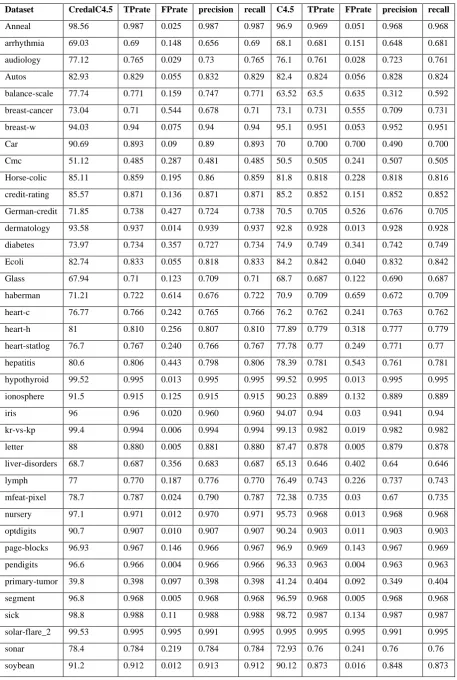
Table 2 Different measures obtained while executing Credal C4.5 with Preprocessed Noisy Dataset

Dataset CredalC4.5 TPrate FPrate precision recall C4.5 TPrate FPrate precision recall

Anneal 98.56 0.987 0.025 0.987 0.987 96.9 0.969 0.051 0.968 0.968

arrhythmia 69.03 0.69 0.148 0.656 0.69 68.1 0.681 0.151 0.648 0.681

audiology 77.12 0.765 0.029 0.73 0.765 76.1 0.761 0.028 0.723 0.761

Autos 82.93 0.829 0.055 0.832 0.829 82.4 0.824 0.056 0.828 0.824

balance-scale 77.74 0.771 0.159 0.747 0.771 63.52 63.5 0.635 0.312 0.592

breast-cancer 73.04 0.71 0.544 0.678 0.71 73.1 0.731 0.555 0.709 0.731

breast-w 94.03 0.94 0.075 0.94 0.94 95.1 0.951 0.053 0.952 0.951

Car 90.69 0.893 0.09 0.89 0.893 70 0.700 0.700 0.490 0.700

Cmc 51.12 0.485 0.287 0.481 0.485 50.5 0.505 0.241 0.507 0.505

Horse-colic 85.11 0.859 0.195 0.86 0.859 81.8 0.818 0.228 0.818 0.816

credit-rating 85.57 0.871 0.136 0.871 0.871 85.2 0.852 0.151 0.852 0.852

German-credit 71.85 0.738 0.427 0.724 0.738 70.5 0.705 0.526 0.676 0.705

dermatology 93.58 0.937 0.014 0.939 0.937 92.8 0.928 0.013 0.928 0.928

diabetes 73.97 0.734 0.357 0.727 0.734 74.9 0.749 0.341 0.742 0.749

Ecoli 82.74 0.833 0.055 0.818 0.833 84.2 0.842 0.040 0.832 0.842

Glass 67.94 0.71 0.123 0.709 0.71 68.7 0.687 0.122 0.690 0.687

haberman 71.21 0.722 0.614 0.676 0.722 70.9 0.709 0.659 0.672 0.709

heart-c 76.77 0.766 0.242 0.765 0.766 76.2 0.762 0.241 0.763 0.762

heart-h 81 0.810 0.256 0.807 0.810 77.89 0.779 0.318 0.777 0.779

heart-statlog 76.7 0.767 0.240 0.766 0.767 77.78 0.77 0.249 0.771 0.77

hepatitis 80.6 0.806 0.443 0.798 0.806 78.39 0.781 0.543 0.761 0.781

hypothyroid 99.52 0.995 0.013 0.995 0.995 99.52 0.995 0.013 0.995 0.995

ionosphere 91.5 0.915 0.125 0.915 0.915 90.23 0.889 0.132 0.889 0.889

iris 96 0.96 0.020 0.960 0.960 94.07 0.94 0.03 0.941 0.94

kr-vs-kp 99.4 0.994 0.006 0.994 0.994 99.13 0.982 0.019 0.982 0.982

letter 88 0.880 0.005 0.881 0.880 87.47 0.878 0.005 0.879 0.878

liver-disorders 68.7 0.687 0.356 0.683 0.687 65.13 0.646 0.402 0.64 0.646

lymph 77 0.770 0.187 0.776 0.770 76.49 0.743 0.226 0.737 0.743

mfeat-pixel 78.7 0.787 0.024 0.790 0.787 72.38 0.735 0.03 0.67 0.735

nursery 97.1 0.971 0.012 0.970 0.971 95.73 0.968 0.013 0.968 0.968

optdigits 90.7 0.907 0.010 0.907 0.907 90.24 0.903 0.011 0.903 0.903

page-blocks 96.93 0.967 0.146 0.966 0.967 96.9 0.969 0.143 0.967 0.969

pendigits 96.6 0.966 0.004 0.966 0.966 96.33 0.963 0.004 0.963 0.963

primary-tumor 39.8 0.398 0.097 0.398 0.398 41.24 0.404 0.092 0.349 0.404

segment 96.8 0.968 0.005 0.968 0.968 96.59 0.968 0.005 0.968 0.968

sick 98.8 0.988 0.11 0.988 0.988 98.72 0.987 0.134 0.987 0.987

solar-flare_2 99.53 0.995 0.995 0.991 0.995 0.995 0.995 0.995 0.991 0.995

sonar 78.4 0.784 0.219 0.784 0.784 72.93 0.76 0.241 0.76 0.76

spambase 93 0.93 0.078 0.93 0.93 92.65 0.922 0.074 0.924 0.922

splice 94.5 0.945 0.026 0.946 0.945 93.71 0.942 0.025 0.944 0.942

sponge 92.1 0.921 0.921 0.848 0.921 91.97 0.921 0.921 0.848 0.921

tae 59.6 0.596 0.201 0.595 0.596 54.3 0.51 0.247 0.507 0.51

vehicle 72.5 0.725 0.093 0.722 0.725 72.43 0.727 0.092 0.724 0.727

vote 96.3 0.963 0.041 0.963 0.963 96.21 0.961 0.047 0.961 0.961

vowel 80.8 0.808 0.019 0.811 0.808 77.48 0.771 0.023 0.776 0.771

waveform 77.3 0.773 0.114 0.773 0.773 75.25 0.748 0.126 0.747 0.748

[image:7.595.67.530.71.514.2]

zoo 93.1 0.931 0.006 0.938 0.931 92.48 0.921 0.008 0.922 0.921

Fig. 5 5%noise

0

10

20

30

40

50

60

70

80

90

100

ann

eal

aud

iol

ogy

balanc

e-scale

breast

-w

cmc

credit

-rati

ng

derm

atology

ecoli

hab

erm

an

heart

-h

hepat

iti

s

ionosphere

kr

-vs

-kp

live

r-disor

ders

mfe

at

-pixe

l

optd

igits

pend

igits

segm

ent

sol

ar

-flar

e_2

soybean

spli

ce

_tae

vote

wav

eform

credal c4.5

[image:8.595.56.528.67.677.2]

Fig. 6 10%noise

Fig.7 20%noise

0

10

20

30

40

50

60

70

80

90

ann

eal

aud

iol

ogy

balanc

e-scale

breast

-w

cmc

credit

-rati

ng

derm

atology

ecoli

hab

erm

an

heart

-h

hepat

iti

s

ionosphere

kr

-vs

-kp

live

r-disor

ders

mfe

at

-pixe

l

optd

igits

pend

igits

segm

ent

sol

ar

-flar

e_2

soybean

spli

ce

_tae

vote

wav

eform

credal c4.5

c-c4.5

0

10

20

30

40

50

60

70

80

ann

eal

aud

iol

ogy

balanc

e-scale

breast

-w

cmc

credit

-rati

ng

derm

atology

ecoli

hab

erm

an

heart

-h

hepat

iti

s

ionosphere

kr

-vs

-kp

live

r-disor

ders

mfe

at

-pixe

l

optd

igits

pend

igits

segm

ent

sol

ar

-flar

e_2

soybean

spli

ce

_tae

vote

wav

eform

credal c4.5

[image:9.595.67.530.69.635.2]

Fig 8. 30%noise

Fig.9 0%noise

The Friedman test is the non-parametric alternative to the one-way ANOVA with repeated measures. It is used to test for differences between groups when the dependent variable being measured is ordinal. It can also be used for continuous data that has violated the assumptions necessary to run the one-way ANOVA with repeated measures. The steps that are involved in this test are;

 Null and Alternative Hypotheses are defined

 Set Alpha value

 Degrees of Freedom is calculated

 Rank the scores of every subject and replace the original values with the ranks

 Calculate chi-square value and using this p-value is determined

0

10

20

30

40

50

60

70

80

ann

eal

aud

iol

ogy

balanc

e-scale

breast

-w

cmc

credit

-rati

ng

derm

atology

ecoli

hab

erm

an

heart

-h

hepat

iti

s

ionosphere

kr

-vs

-kp

live

r-disor

ders

mfe

at

-pixe

l

optd

igits

pend

igits

segm

ent

sol

ar

-flar

e_2

soybean

spli

ce

_tae

vote

wav

eform

credal c4.5

c-c4.5

0

10

20

30

40

50

60

70

80

90

100

credal c4.5

The Credal C4.5 algorithm executed using preprocessed dataset has Statistically significant with p-value of 0.009168 obtained using Wilcoxon Signed Rank Test and 0.039 obtained using Friedman Test.

5.

CONCLUSION

The two most significant issues that are experienced in decision tree algorithms are over fitting which is one of the most practical complexities for decision tree models gets solved by setting constraints on model parameters and pruning and not fit for continuous variables; while working with continuous numerical variables, decision tree loses information when it categorizes variables in different categories. The proposed idea is defined in the way of overcoming the problem addressed in which it minimize the tree size and improves the accuracy level of the algorithm compared to the existing algorithms. In this process, dataset is collected and preprocessed in which noise is also added to the dataset. Preprocessed data undergone CfsSubsetEval feature selection technique and the most relevant features are selected. Then the selected attributes are given as input to the Credal c4.5 algorithm in which decision tree is constructed. This process is carried out for all 50 datasets that are downloaded from UCI repository. The results obtained are compared with the existing algorithm by the accuracy and other statistics. Accuracy and the performance of the algorithm are improved in which the objective is satisfied. The future aim of this work is to implement c5.0 algorithm with imprecise probability function.

6.

REFERENCES

[1] Jose A. Saez, Mikel Galar, Julian Luengo and Francisco Herrera.2013.Tackling the problem of classification with noisy data using Multiple Classifier Systems: Analysis of the performance and robustness. Information Sciences.

[2] Carlos J. Mantasand JoaquinAbellan.2014.Credal-C4.5: Decision tree based on imprecise probabilities to classify noisy data. Expert Systems with Applications, 4625– 4637.

[3] Joaquin Abellan and Javier G. Castellano.2017.A comparative study on base classifiers in ensemble methods for credit scoring, Expert Systems with Applications, 1–10.

[4] Yisen Wang, Shu-Tao Xia and JiaWu .2016.A less-greedy two-term Tsallis Entropy Information Metric approach

for decision tree classification. Knowledge-Based Systems, 1–9.

[5] Dewan Md. Farid, Mohammad Abdullah Al-Mamun and Bernard Manderick, Ann Nowe.2016.An adaptive rule-based classifier for mining big biological data. Expert Systems With Applications, 64, 305–316.

[6] FarhadPourpanah, CheePeng Limb and Junita MohamadSaleh. 2015.A hybrid model of fuzzy ARTMAP and genetic algorithm for data classification and rule extraction. Expert Systems With Applications . [7] AbeerM.Mahmoud.2016.Suitability of Various Intelligent

Tree Based Classifiers for Diagnosing Noisy Medical Data. Egyptian Computer Science Journal Vol. 40 No.2 .

[8] Hong Zhao and Xiangju Li. 2016.A cost-sensitive decision tree algorithm based on weighted class distribution with batch deleting attribute mechanism. Information Sciences, 1–14 .

[9] Carlos J. Mantas, JoaquinAbellan and Javier G. Castellano.2016.Analysis of Credal-C4.5 for classification in noisy domains. Expert Systems With Applications, 61, 314–326

[10] Moloud Abdar , Mariam Zomorodi-Moghadam , Resul Das and I-Hsien Ting.2016.Performance analysis of classification algorithms on early detection of Liver disease. Expert Systems With Applications.

[11]Jinghua Liu, Yaojin Lin, Menglei Lin, Shunxiang Wu and JiaZhang.2016.Feature selection based on quality of information. Neurocomputing.

[12]Jose A. Saez, Mikel Galar, Julian Luengo and Francisco Herrera.2013.Tackling the problem of classification with noisy data using Multiple Classifier Systems: Analysis of the performance and robustness. Information Sciences.

[13] Abeer M.Mahmoud.2016.Suitability of Various Intelligent Tree Based Classifiers for Diagnosing Noisy Medical Data. Egyptian Computer Science Journal Vol. 40 No.2.