Generalizations of Rough Functions in Topological Spaces
by Using Pre-Open Sets
Amgad S. Salama1, Hassan M. Abu-Donia2
1Department of Mathematics, Faculty of Science, Tanta University, Tanta, Egypt; 2Department of Mathematics, Faculty of Science,
Zagazig University, Zagazig, Egypt.
Email: {dr_salama75,donia_1000}@yahoo.com
Received January 25th,2011; revised March 6th, 2012; accepted March 14th, 2012
ABSTRACT
Functions are a means to link or transport from a world to another world may be similarly or completely different from the other world. In this paper we addressed the issue of rough functions and the possibility of transfer it from the real line to the topological abstract view that can be applied to intelligent information systems. The rough function approach has not been studied much specially from a topological point of view. Here we developed a new type of topological generalizations of rough functions with reference to how it is used in medical applications. Considering that the func- tion is in the original a relation can be based on a review of all circular functions from the perspective of relations. Ac- cordingly, the dream that the generalizations of rough functions are transferred to all papers prior to a comprehensive computer application.
Keywords: Rough Sets; Rough Numbers; Approximation Spaces; Topological Spaces; Fuzzy Sets
1. Introduction
Rough set theory [1], is an extension of set theory for the study of intelligent systems characterized by inexact, un- certain or insufficient information. Moreover, this theory may serve as a new mathematical tool to soft computing besides fuzzy set theory [2-4], and has been successfully applied in machine learning, information sciences, expert systems, data reduction, and so on. Recently, lots of re- searchers are interested to generalize this theory in many fields of applications [5-7]. In classical rough set theory, partition or equivalence (indiscernibility) relation is an important and primitive concept. But, partition or equi- valence relation is still restrictive for many applications. To study this issue, several interesting and meaningful generalizations to equivalence relation have been pro- posed in the past, such as tolerance relations [8], topo- logical bases and subbases [9-12]. Particularly, some researchers have used coverings of the universe of dis-course for establishing the generalized rough sets by co-verings [13]. Others [14-16] combined fuzzy sets with rough sets in a fruitful way by defining rough fuzzy sets and fuzzy rough sets. Furthermore, another group has characterized a measure of roughness of a fuzzy set making use of the concept of rough fuzzy sets [17-19]. They also suggested some possible real world applica- tions of these measures in pattern recognition and image analysis problems. Some results of these generalizations
are obtained about rough sets and fuzzy sets in [20-22]. Topological ideas are present not only in almost all areas of today mathematics, for example biochemistry [23] information systems [24] and others for more fields of topology applications [25] and its related links. The sub- ject of topology itself consists of several different bran- ches such as point set topology, algebraic topology and differential topology which have relatively little in com- mon this richness of applications and differentiate be- tween branches of topology implied a difficult to give an accurate definition for topology. The topology concepts like continuity, irresoluteness, compactness, connected- ness, convergence, denseness and others are as basic to mathematicians. The topology structure τ on a set X is a general tool for constructing the above concepts. This tool contains many classes of near open sets such as: regular open [26], semi open sets [27], pre-open sets [28], β-open sets [29] and b-open sets [30]. Many authors used the previous types of near open sets to introduce some types of near continuous functions such as: In [28] the concept of pre-continuous functions are introduced. In [31] the concept of α-continuous functions is introduced.
study on rough functions and to introduce some concepts based on rough functions. In the beginning we will study rough sets on the real line.
In Section 2, we will initiate the notion of rough real functions. The aim of Section 3 is to define and study the new notion of “topological pre-rough function”. The main goal of Section 4 is to initiate and study the pre-appro- ximations of a function as a relation. Finally, we aim in Section 5 to define an alternative description of the topo- logical pre-rough functions and topological pre-rough con- tinuity.
A topological space [36] is a pair consisting
of a set X and family τof subsets of X satisfying the fol-lowing conditions:
( , )X τ
1) φ, Xτ.
2) τis closed under arbitrary union. 3) τis closed under finite intersection.
The pair is called a topological space, the
elements of X are called points of the space, the subsets of X belonging to are called open set in the space, and the complement of the subsets of X belonging to τ be called closed set in the space; the family τof open subsets of X
is also called a topology for X.
( , )X τ
= : , c
A FX AF Fτ
is called τ-closure ofa subset AX.
Evidently, A is the smallest closed subset of X which contains A. Note that A is closed iff A= A.
= : ,
A GX GA Gτ
is called the τ-interior of a subset AX.Evidently, A is the union of all open subsets of X which containing in A. Note that A is open iff A=A. And b A( ) =AA is called the τ-boundary of a subset
AX .
Let A be a subset of a topological space ( , )X τ . Let
A, A and be closure, interior, and boundary of
A respectively.
( ) b A
A is exact if , otherwise A is
rough. It is clear A is exact iff b A( ) =A= Aφ.
Definition 1.1: A subset A of a topological space
is called pro-open if
( , )X τ Aint cl A
( )
.The family of all pre-open sets of X is denoted by
. The complement of pre-open set is preclosed
set. The family of preclosed sets is denoted by .
( ) PO X
( ) PC X , )σ
Definition 1.2: A function is said
to be pre-continuous if f1f( )G: ( ,XPO Xτ)( )(Y for every
[28].
Gσ
2. Rough Functions on Real Line
Let be the set of non-negative real numbers, and let
be a sequence of real numbers defined by
1 2 3 such that 1 2 3 .
The sequence defines the partition of
R R , ,x
Seq
,
x x , ,xn Seq
< < < < n <
x x x x
π(Seq) R
by 1 1 1 2 2 1 ,
where 1
, ), , ,( ,x x x xi i ),
π(Seq) ( ,
= 0,(0, )
i i
), ,( x x x x x
q
denote open intervals . The
se-quence is called a categorization of
R R
Se and the
ordered pair A=
R,π*(Seq)
*
π (Seq) (Seq)
is an approximation
space, where is the equivalence relation
asso-ciated with π .
Let A=
R,π*(Seq)
be an approximation space.By Seq x( ) in A we denote the block of the partition containing x, in particular if
π(Seq) x Seq , we have
x ( )x =Seq , clSeq x
is the closure of with respect to the usual topology on R. Let( )x *
π
Seq
=
, ( )
A R)
Seq (
be an approximation space, by Q x we denote the
closed interval [0, ]x for x R . For any x R
)
, the
Seq-lower and the Seq-upper approximations of
in the approximation space
( ) Q x =
,π*(
A R Seq are
de-fined respectively by
* ( )
Seq Q( )x = y R :Seq y( )Q x
φ
Q x *
( ) = Seq Q( )x = y R :Seq y( )Q x
The approximations of the closed interval
can be understood as the approximations of the real number
( ) = [0, ]x
x which are simply the ends of the interval
. The number
( )
Seq x x is a rough number if
* , otherwise it is an exact
number.
( )x Seq Q x*
( )
R =
Seq Q
Example 2.1: Let be the set of all non-negative
real numbers, and let be the set of
nat-ural numbers to be a sequence in . Then the partition
induced by is
= {1, 2,3,
N }
R N
π( ) = 0,N (0,1),1,(1, 2), 2, , ,( n n n, 1),n1,
and hence, A=
R,π*( )N
is an approximation space.Also, for any number x N , we have and
for any
( ) = { N x x} x N , N x( ) =
x xi, i1
and x
x xi, i1
,Then every number x N is a rough number in A. According to Example 1, we followed the following
steps to get the approximations of a number x, say
. We remark that the required approximations of can be obtained directly in one step by
= 1.2 x
= 1.2 x
(1.2)
=N
1.2Bnd Q .
Let X and Y be two subsets of R, and let A= ( , )X S
S
and be two approximation spaces, where
and P are equivalence relations on X and Y, respectively,
= ( B Y, )P
:
f X Y is a function. Then we define -lower
approximation of
( , )S P f as the function f*:X Y, such
that f x*( ) =P f x*
( )
for every x X , and (S, P)-upper approximation of f as the function f*:X Y,
such that f x*( ) =P f x*
( )
, for every x X .We see that the term
S P,
in the above definitioncan be replaced by P only since the approximations of
the function f depends only on P.
Let f X: Y
R
be a real valued function, where X and
Y are two subsets of . The function f is called a rough
function at a point x X if and only if *
*( ) = ( )
f x f x
and f is called a rough function on X if it is a rough function at every point x X .
We give the following example to indicate the above notions.
ction defined by f x( ) =x1 for every x R . We de-note the odd and even integers by O and E, respectively, then A=
R ,π
R
π( ) = 0,(E O
π π
0,1),1,(1,3),and are ap-
proximation spaces, where and are
parti-tions of defined by
and , then at every point
π* Eπ( )E
(0,1),1,(
= ,
B R ( )O
( ) = 0,O 1,3),
x R
*:
we define E-lower approximation of f by
f RR
such that
( )* 0, 1
E x
E y x
*= * =
:
f E f x
y R
1 =E* 0 x
, 1
=
*:
and the E-upper approximation of f by the function
f RR * =E f
= 3 x
such that
* .
For , we have
= :
x y R
(3) = 3 f
φ
( ) E y( ) [0
1 = 4
,x1] = f x
, then
*= 0, 4
0, 4 = 0,
( ) 0, 4 =
E y y φ
* 3 = * 4
:
= :
f E
y R E
y R E
4= 0, 4 =
.
and 4 =E*
0,
4* 3 = *
f E = 3 x = 2 x
. Then f is an exact fun-
ction at , similarly we can prove that f is an exact
functional at every odd natural number.
For , then
* = 0,3: ( ) 0,3
E
E y
= 0, 2* 2 = * 3
=
f E
y R
But
* = 0,3: ( ) 0,3
E E y
= φ
= 0
, 4* 2 = * 3
=
f E
y R
Then f is a rough function at , similarly it
can be proved that
= 2
x
f is a rough function at every even natural number.
Also, we notice that f is a rough function at every
x N . Then f is a rough function at every point
x N or x is an even natural number.
Let f X: Y be a real valued function. Then f
is called ( , -continuous (roughly continuous) at a
point
)
S P
x X if f clS x
*
P f x , where
= ( , )
A X S
: and B= ( , )Y P are approximation spaces.
Let f X Y be a real valued function. Then f
is roughly continuous on X if f is a roughly
con-tinuous at every point x X .
Example 2.3: According to Example 2, the function
:
f R R
lS 1.5 =
is a rough function at
2, 4
x= 1.5 butf c and P f*
1.5 =
E*
2.5 = 0, 4
= 1
x
,
then f is not a rough continuous function at the rough
number x= 1.5, but at , since f clS
1 = 2
and E*
f
1 =
0, 2 then f is a roughly continuous at, also at every = 1
x x N
R
such that x is odd number f
is roughly continuous. If x is an even number, then f is not a roughly continuous; hence f is not a roughly
con-tinuous function on .
Example 2.4: Let X and Y be subsets of R, such that
= 1,3,5,7
X and Y= 2, 4,6
and the real valuedfunction f X:
(7) f = ( , Y = 6 )
be defined by ,
and , and consider the
approxima-tion spaces
(1) = (5) = 2
f f
(3) = 4
f
A X S and B= (Y, )P , where
\ =*:
\ = 1,5 ,
X S 3,7 and Y P we de-
fine the function
2 , 4,6
f XY by f x*
=P f x*
.Then,
*(1) = *(2) = {2}
f P
(5) = (2) = {2}
f P
, f*(3) =P*(4) =φ,
(7) = (6) =
f P φ
* * , * * .
Also for the function f*:X Y such that
* = *
f x P f x
*(3) = *(4) = {4, 6
f P
. Then, * *(2) = {2},
*(5) = *(2) = {2}
f P
(1) =
f P
}
*(7) = *(6) = {4, 6}
f P
, ,
. Then the function f is P-rough at
and f is not P-rough function at .
= 3.7
x x= 1.5
Now, if x= 1, then Seq x
=clSeq x
= 1,5 and we have f clSeq x
= f
1,5 = 2
and
= 2
* =P* 2
P f x ,
then f clSeq x
P*
f
x
, i.e., the function f is
x= 3
x
,
S P -roughly continuous at = 1.
If , then Seq x
=clSeq
x
= 3, 7
and
4,6f 3,7 = , but P*
f x
=P*
4 = 4,6
then, the function f is
S P,
= 5.7
,-roughly continuous at
. Also at we find that f is -rough-
ly continuous, hence f is = 3
x x S P
S P,
-roughly continuous onX.
3. Topological Pre-Rough Functions
We purpose to generalize the concept of rough function to topological pre-rough function by using pre-open sets in topological spaces. Let
X,τ
be a topological space and x X . Then pmin
x =
G PO X
:x G
iscalled the pre minimal set containing the point x with
respect to pre-open sets in the topology on τ X.
The principle topology on a set X is the topology has the minimal bases that consists only of minimal open sets at each x X .
Theorem 3.1: A topology on a set X is principle iff
arbitrary intersections of members of are members of [20].
τ
τ τ
Let
X,τ
be a principle topological space, for anyelement x X , we define pre-sequence by the set
,
Seq x = G:G PO X x G and by pSeq x
we mean the pre-closure of Seq x
in
X,τ
.If f :
X,τ
Y,σ
is a function between principle spaces
X,τ
and
Y,σ
, we define the functions
: , ,
f
n X τ Y σ
pmi , by
= { : O
n xf G G P and
pmi Y f x G for
every
x X
, and pclf :
X,τ
Y,σ
, by
=
f σ
pcl x pcl f x for all x X .
Let f : ,
X τ
Y,σ
be a function, where X andfunction on X if it is a topological pre-rough function at every point x in X.
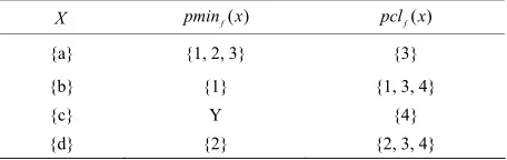
Example 3.1: Let and be topological
spaces, where
,
X τ
= , , ,
,
Y σ
X a b c d
,
,d , ,c
= , , , , , ,
τ X φ a a d a c d
= 1, 2,3, 4
Y
, c , d , ,a c
and , σ =
Y, , 1 , 2 , 1, 2 , 1, 2,3φ
: , ,
f X τ Y σ
.Let be a map defined by f a
= 1f b f c
= 4= 3,
, and f d
= 2. We have thefol-lowing table (Table 1).
Consequently, pmin xf
= pcl xf
for every x X , hence f is a topological pre-rough function on X.A function is said to be a
topo-logical pre-rough continuous at the point
: , ,
f X τ Y σ
x X if and
only if
p
σ
f Seq x pcl Seq f x , and it is a topological pre-rough continuous on X if it is a topo-logical pre-rough continuous at every point x X .
Example 3.2: Let and be topological
spaces, where
,
X τ
= , , ,
,
Y σ
X a b c d
, , , ,a b a
, 1, 2, 4
and with
and
= 1, 2,3, 4
Y
= , , ,
τ X φ c
= , , 1 , 1
σ Y φ
,a b b
, 4 . Let
,
= 2f b
: ,
f X τ Y σ
be a map defined by f a
= 1, , f c
= 4and f d
= 3 (Table 2).Consequently,
p
σ
f Seq x pcl Seq f x for every x X , hence f is a topological pre-rough con-tinuous function on X.
4. The Pre-Approximations of Functions
A function f from X to is a relation from Y X to that satisfies:
Y
1) Dom f
= X .
,2) If x y f and
x z, f , then y=z.If X = , we say Y f is a function on X. A function :
f X Y
= ,is completely represented by its graph
:
g f x f x xX .
[image:4.595.59.287.556.628.2]The concept of rough relations is defined by using a certain type of relation products. The following proposition
Table 1. pmin xf( ) and pcl x for some subsets of X. f( )
X pmin xf( ) ( )pcl xf
{a} {1, 2, 3} {3}
{b} {1} {1, 3, 4}
{c} Y {4}
{d} {2} {2, 3, 4}
Table 2. Topological pre-rough continuous function on X.
X Seq(x) pSeq x( ) f
pSeq x( )
( )
σ
pcl Seq f x
{a} {a} {a, c, d} {1, 3, 4} Y
{b} {b} {b, c, d} {2, 3, 4} Y
{c} {a, b, c} X Y Y
{d} {a, b, d} X Y Y
will simplify the process of getting
U U1 2
R1R2
via
U R1 1
and
U R2 2
.Theorem 4.1: Let A1=
U R1, 1
and A2 =
U R2, 2
be a pre-approximation spaces. Then we have
U U1 2
R1R2
= U R1
U R2 2
Proof: Since for any and 2
1
1
,
u uU
. ,
v vU , we
have,
u v, , u v ,
R1.R2 iff
u u,
R1 and
v v,
R2 . Let
1 2 1 2 1 2
, (
u v
U ) R R
R R
U ( ).
Then we have
1 2
1 2
1 2
1 2
1 2
, , : , , ,
= , : , and , = : , : , =
R R
R R
u v u v u v u v R R
u v u u R v v R
u u u R v v v R
u v
.
Hence
U U1 2
R1R2
= U R1 1
U R2 2
. Let f :
U R1, 1
U R2, 2
be any function, where
1 = 1, 1
A U R and A2 =
U R2, 2
R R
2 U
1 2 =
R R R
are pre-approximation spaces, such that 1 and 2 are equivalence relations on 1 and respectively. We define the equivalence rela-
tion
U
such that
1 2
1 R1
U R2
is a partition of1 2
2
=
U U R U
U U for the function g f
=
x f x,
:x U 1
we define the pre-approximations
=
1, 2
1 2:
1, 2
pR g f u u U U u u Rg f
=
1, 2
1 2:
1, 2
=
pR g f u u U U u u Rg f φ
A function f : U1U2 is said to be roughly in the pre-approximation space A=
U2, R
, where
1= 1, 1
A U R and A2 =
U2, R2
1 2
are pre-approxima-
tion spaces and A= AA , U2 =U if
1U2
=
pR g f R g f p
, otherwise f is pre-exact function.
Example 4.1: Let U1 =
a b c d e, , , ,
and
2 = 1, 2,3, 4,5,6
U
1 2
:
and consider the function
f U U defined by
, ,5 , , 2 , ,3c d e
( ) = ,3 , ,6
g f a b .
Consider the partitions U R1 1=
a c, ,
b , d e,
and
2 2= 1 , 2,5 , 3, 4 , 6
U R . Then
1 2 1 1 2 2
=
,1 , ,1 , , 2 , , 2 , ,5 , ,5 ,
,3 , , 4 , ,3 , , 4 , ,6 , ,6 ,
= ,1 , , 2 , ,5 , ,3 , , 4 , ,6 ,
,1 , ,1 , , 2 , ,5 , , 2 , ,5 ,
,3 , , 4 , ,3 , , 4 , ,6 , ,6
U U R U R U R
a c a c a c
a a c c a c
b b b b b b
d e d d e e
d d e e d e
[image:4.595.56.288.655.736.2]Then pR g f
=
b,6
and
,3 , , 4 , ,3 , , 4 , ,6 , , 2 ,
= , 2 , ,5 , ,5 , , 2 , ,5 , , 2 ,
,5 , ,3 , , 4 , ,3 , , 4
p
a a c c b a
R g f c a c d d e
e d d e e
Therefore the function f is a rough function such that
=p
pR g f R g f .
For the function f U: 1U2, we observe that in
general pR g f
and
pR g f are not functions
from into . We point that, the process of
de-fining an pre-approximations on
such that1
U U2
1 2
U U
f
pR g and R g
f
p are functions is an open
question to be solved in our next work.
Theorem 4.2: For every function f U: 1U2 such
that A1=
U R1, 1
and A2 =
U R2, 2
are selective pre-approximation spaces then f is an pre-exact function.
Proof: Since in any selective pre-approximation space,
R
x y, =
x,
y then pR g f
=p R g f
then f is an preexact function.
Example 4.2: Let U1=
a b c d, , ,
and U2 = 1, 2,3
.Consider the function f U: 1U2, defined by g f
=
a,1 , ,1 , , 2 ,b c
d,3
and consider the partitions
= ,
U R1 1
a b , c
, d
and U R2 2= 1 , 2 , 3
.Then
1 2 = 1 1 2 2 =
,1 , , 2 , ,3 , ,1 , , 2 , ,3 ,
,1 , , 2 , ,3 , ,1 , , 2 , ,3
U U R U R U R
a a a b b b
c c c d d d
is a partition of U1U2.
Then pR g f
=
a,1 , ,1 , , 2 , ,3b c d
and
=
,1 , ,1 , , 2 , ,3
pR g f a b c d , then f is an
pre-exact function.
For a function f U: 1U2 such that A1=
U R1, 1
and A2 =
U R2, 2
are selective pre-approximation spa- ces then1) If f is a one-to-one function then also both
pR g f
and
pR g f .2) If f is onto function then also both pR g f
and
pR g f .
3) If f is a pre-continuous function then also both
pR g f
and
pR g f .No function f U: 1U2 such that A1=
U R1, 1
and A2 =
U R2, 2
are not selective approximation spaces is pre-exact, and f is not a constant function.5. An Alternative Description of Topological
Pre-Rough Functions
Let
U1,τ1
and
be any topological spaces,the function
we define p f = pint f
and pf = pcl f
for the function f. Let f :
U1,τ1
U2,τ2
be a function,where
U1,τ1
and
U2,τ2
, are topological spaces,the function f is called a topological pre-rough function in
U U1 2,τ
iff =p
pf f otherwise, f is an preexact
function in
1 2 τ
Example 5.1: Let
, U U .
U1,τ1
1
U
and be any
to-pological spaces where ,
U2,τ2
,
= a b c,
2 = 1, 2,3, 4
U , τ1=
U1, ,φ
a , , ,b c d
,
2= 2, , 3 , 1, 2, 4
τ U φ Consider β1=
a , , ,b c d
and β2= 3 , 1, 2, 4
:are basis of and res-
pectively. Let
1
τ τ2
1 2
f U U , g U: 1U2 and
are mappings defined by
1 2
:
h U U
= ,3 , ,1 , , 2 , , 4
f a b c d ,
= , 2 , ,3 , ,1 , , 4
g a b c d
and h=
a,3 , ,3 , ,3 , ,3b c d
. Then pf = pinf f
=
a,3 and
,3 , ,1 , , 2 , , 4 , ,1 ,
= =
, 2 , , 4 , ,1 , , 2 , , 4
pf cl f a b b b c
c c d d d
Then f is a pre-rough function in
U U1 2,τ
. Also,
= =
pg pint g φ and =
= 1 2 pg pcl g U UWe call g is a function not defined from pre-lower and from upper. Finally, for the constant function h, we have
= ( ) = ( ) =p
ph pint h pcl h h, and h is an pre-exact
func-tion. In fact, h is the only exact function in
U U1 2,τ
. According to Example 1, we have the following: 1) The function f is continuous, but p f and p f arenot functioning, hence we cannot say that f or f is
pre-continuous.
2) The function h is always precontinuous function,
and it is an pre-exact function, hence ph and ph is
pre-continuous functions.
6. Experiments and Evaluations
This section shows the effectiveness of using pre-rough functions for extracting new data from multi-valued in-formation systems.
2, 2
U τ
U2,τ2
1
: 1, 1
f U τ
1 2
U U , can be considered
as a relation of and if β is a basis of 1 and
2
τ β is a basis of τ2, then β=β1β2 is a basis of the
topology on τ U U1 2. In the topology
U U1 2,τ
age 3-5 years. This disease has many symptoms and it is usually started in young age and still with the patient along his life.
Table 3 in [37] introduced the seven patients charac-
terized by 8 symptoms (attributes) using them to decide the diagnosis for each patient (decision attribute). Where the attributes are satisfied in Table 2 in [37].
We recall and sell it here Table 3.
If we defined the following mapping on Table 3:
: ( )
f UP U :
( 1) 1, 2 , 2 2, 3
f p p p f p p p ,
( 3) { 3}, ( 4) { 2, 4}, ( 5) { 1, 5, 7}
f p p f p p p f p p p p
( 6) { 6}, ( 7) { 5, 7}
f p p f p p p
From the relation where
a is an element of the power set of the set of condition
attributes . The the following classes
a
{( , ) : ( ) ( )}
a a a
R x y f x f y
α β δ, ,
1 :
χ xR x U and χ2
R x x Ua :
are twosubbases of two topologies on U such that
a a . Then according to Table 3 we have
the following couples of topologies:
:yR x
R x y
2 3 2 3 1 2
1 1 2 3 2 3 4 5 6 7
1 2 4 5 6 7 2 4 5 6 7
, , , , , , , ,
, , , , , , , , ,
, , , , , , , , , ,
α
U φ p p p p p p
τ p p p p p p p p p
p p p p p p p p p p p
,
1 3 1 3 4 5 6 7
2 3 4 5 6 7 1 4 5 6 7
1 2 4 5 6 7 2 3 4 5 6 7
, , , , , , , , , ,
, , , , , , , , , ,
, , , , , , , , , , ,
α
U φ p p p p p p p p
τ p p p p p p p p p p
p p p p p p p p p p p p
5 7 3 7 1 4
1 5 7 3 5 7 1 4 5
1 4 5 7 1 2 4 6
, , , , , , , ,
, , , , , , , ,
, , , , , , ,
β
U φ p p p p p p
τ p p p p p p p p
p p p p p p p p
3 5 7 2 3 6 2 3 6 7
1 2 4 6 1 2 3 4 6
2
2 3 5 6 7 1 2 4 5 6
1 2 3 4 5 6 1 2 3 4 6 7
, , , , , , , , , , , ,
, , , , , , , , ,
, , , , , , , , , ,
, , , , , , , , , , ,
β
U φ p p p p p p p p p p
p p p p p p p p p
τ
p p p p p p p p p p
p p p p p p p p p p p p
4 5 2 7 4 5
1 2 4 7 2 5 7 2 4 5 7
1 2 3 5 6 7
, , , , , , , ,
, , , , , , , , , ,
, , , , , δ
U φ p p p p p p
τ p p p p p p p p p p
p p p p p p
4 1 3 6 1 3 4 6
1 3 5 6 1 2 3 6 7
2
1 2 3 5 6 7 1 3 4 5 6
1 2 3 4 6 7
, , , , , , , , , ,
, , , , , , , , ,
, , , , , , , , , , ,
, , , , ,
δ
U φ p p p p p p p p
p p p p p p p p p
τ
p p p p p p p p p p p
p p p p p p
1 1 1 { , }
αβ α β
τ τ τ U φ
2 2 2 { , }
αβ α β
τ τ τ U φ
1αδ 1α 1δ { , }
τ τ τ U φ
2 2 2
1 1 1 5
2 2 2 1 2 3 4 6 7
1 1 1 1
2 2 2 2
{ , } { , ,{ }}
{ , ,{ , , , , , }} { , }
{ , } αδ α δ
βδ β δ
βδ β δ
α β δ α β δ
α β δ α β δ
τ τ τ U φ
τ τ τ U φ p
τ τ τ U φ p p p p p p
τ τ τ τ U φ
τ τ τ τ U φ
According to the mapping and using
each one of the above topologies we can deduce that the decision topology can be given by:
) ( :U PU
f
} , { }, { }, { }, , , , , { , ,
{U p1 p2 p3 p6 p7 p4 p5 p4 p5
D
.
Now we can construct a familiar system of Table 3
contains only the pre-rough images constructed using the terminology of pre-rough functions. This system can be the reduction system of Table 3 and it given in Table 4.
This means that we can remove the conditional attrib-ute {}without any loss of information.
7. Conclusions
We conclude that the emergence of topology and its op-erators [38,39] in the construction of some rough set concepts will help to get rich results that yields a lot of logical statements which discover hidden relations be-tween data and moreover, probably help in producing
Table 3. Multi-valued information system of [37].
D δ β α U
p1 { }α2 { , , }β β1 2 β4 { }δ1 {d3}
p2 { , }α α1 2 { , }β β1 2 { , }δ δ1 3 {d3}
p3 { }α3 { , }β β1 3 { }δ1 {d3}
p4 { }α1 { , , }β β β1 2 4 { }δ4 {d1}
p5 { }α1 { }β5 { , }δ δ1 2 {d2}
p6 { }α1 { , }β β1 2 { }δ1 {d3}
p7 { }α1 { , , }β β β1 3 4 { , }δ δ1 3 {d3}
Table 4. Reduced System.
U β δ
p1 { , , }β β β1 2 4 { }δ1
p2 { , }β β1 2 { , }δ δ1 3
p3 { , }β β1 3 { }δ1
p4 { , , }β β β1 2 4 { }δ4
p5 { }β5 { , }δ δ1 2
p6 { , }β β1 2 { }δ1
accurate programs. These topological operators will play an essential role in data mining and knowledge discovery in databases. In this paper, we give an overview of sev-eral dissipated results on the pre-rough functions. More specifically, we attempt to show: usefulness of this new concept in a calculus of rough functions.
The future application of this work will be useful in many fields such as Fuzzy Expert Systems [40] by gen-eralizations of rough functions for fuzzy rough functions. It also is useful in knowledge discovery methods [41].
REFERENCES
[1] Z. Pawlak, “Rough Sets,” International Journal of Paral-lel Programming, Vol. 11, No. 5, 1982, pp. 341-356.
doi:10.1007/BF01001956
[2] X. Wang, E. C. C. Tsang, S. Zhao, D. Chen and S. Yeung, “Learning Fuzzy Rules from Fuzzy Samples Based on Rough Set Technique,” Information Sciences, Vol. 177, No. 15, 2007, pp. 4493-4514.
doi:10.1016/j.ins.2007.04.010
[3] S. Zhao and E. C. C. Tsang, “On Fuzzy Approximation Operators in Attribute Reduction with Fuzzy Rough Sets,” Information Sciences, Vol. 178, No. 16, 2008, pp. 3163-3176.
[4] L. A. Zadeh, “Fuzzy Sets,” Informationand Control, Vol. 8, No. 3, 1965, pp. 338-353.
doi:10.1016/S0019-9958(65)90241-X
[5] Z. Bonikowski, “Algebraic Structures of Rough Sets,” In: W. Ziarko, Ed., Rough Sets, Fuzzy Sets and Knowledge Discovery, Springer, London, 1994, pp. 243-247.
doi:10.1007/978-1-4471-3238-7_29
[6] E. Bryniaski, “A Calculus of Rough Sets of The First Order,” Bulletin of the Polish Academy of Sciences, Vol. 16, 1989, pp. 71-77.
[7] Y. Y. Yao, “Constructive and Algebraic Methods of The-ory of Rough Sets,” Information Sciences, Vol. 109, No. 1-4, 1998, pp. 21-47.
doi:10.1016/S0020-0255(98)00012-7
[8] A. Skowron and J. Stepaniuk, “Tolerance Approximation Spaces,” Fund Information, Vol. 27, No. 2-3, 1996, pp. 245-253.
[9] E. F. Lashin, A. M. Kozae, A. A. Abo Khadra and T. Medhat, “Rough Set Theory for Topological Spaces,” In-ternational Journal of Approximate Reasoning, Vol. 40, No. 1-2, 2005, pp. 35-43. doi:10.1016/j.ijar.2004.11.007
[10] K. Qin and Z. Pei, “On the topological Properties of Fuzzy Rough Sets,” Fuzzy Sets and Systems, Vol. 151, No. 3, 2005, pp. 601-613. doi:10.1016/j.fss.2004.08.017 [11] A. Wasilewska, “Topological Rough Algebras,” In: T. Y.
Lin and N. Cercone, Eds., Rough Sets and Data Mining, Kluwer Academic Publishers, Boston, 1997, pp. 425-441.
doi:10.1007/978-1-4613-1461-5_21
[12] W. Zhu, “Topological Approaches to Covering Rough Sets,” Information Sciences, Vol. 177, No. 15, 2007, pp. 1499-1508. doi:10.1016/j.ins.2006.06.009
[13] T. J. Li, Y. Leung and W. X. Zhang, “Generalized Fuzzy
Rough Approximation Operators Based on Fuzzy Cover-ings,” International Journal of Approximate Reasoning, Vol. 48, No. 3, 2008, pp. 836-856.
doi:10.1016/j.ijar.2008.01.006
[14] R. Biswas, “On Rough Sets and Fuzzy Rough Sets,” Bul-letin of the Polish Academy of Sciences, Vol. 42, 1992, pp. 343-349.
[15] G. Liu, “Generalized Rough Sets over Fuzzy Lattices,” Information Sciences, Vol. 178, No. 6, 2008, pp. 1651- 1662. doi:10.1016/j.ins.2007.11.010
[16] A. M. Rolka and L. Rolka, “Fuzzy Rough Approxima-tions of Process Data,” International Journal of Ap-proximate Reasoning, Vol. 49, No. 2, 2008, pp. 301-315.
doi:10.1016/j.ijar.2007.03.016
[17] M. Banerjee and S. K. Pal, “Roughness of a Fuzzy Set,” Information Sciences, Vol. 93, No. 3-4, 1995, pp. 235- 246. doi:10.1016/0020-0255(96)00081-3
[18] R. Biswas, “On Rough Fuzzy Sets,” Bulletin of the Polish Academy of Sciences, Vol. 42, 1994, pp. 352-355. [19] D. Dubois and H. Prade, “Rough Fuzzy Sets and Fuzzy
Rough Sets,” International Journal of General Systems, Vol. 17, No. 2-3, 1990, pp. 191-208.
doi:10.1080/03081079008935107
[20] C. Degang, Y. Wenxia and Li Fachao, “Measures of General Fuzzy Rough Sets on a Probabilistic Space,” In-formation Sciences, Vol. 178, No. 16, 2008, pp. 3177-3187.
doi:10.1016/j.ins.2008.03.020
[21] Z. Gong, B. Sun and D. Chen, “Rough Set Theory for the Interval-Valued Fuzzy Information Systems,” Informa-tion Sciences, Vol. 178, No. 8, 2008, pp. 1968-1985.
doi:10.1016/j.ins.2007.12.005
[22] Y. Yang and C. Hinde, “A New Extension of Fuzzy Sets Using Rough Sets: R-Fuzzy Sets,” Information Sciences, Vol. 180, No. 3, 2010, pp. 354-365.
doi:10.1016/j.ins.2009.10.004
[23] P. Bhattacharya and B. K. Lahiri, “Semi Generalized Closed Sets in Topology,” Indian Journal of Mathematics, Vol. 29, 1987, pp. 373-382.
[24] A. Skowron, “On Topology Information Systems,” Bulle-tin of the Polish Academy of Sciences, Vol. 3, 1989, pp. 87-90.
[25] Z. Pawlak, “Rough Sets: Theoretical Aspects of Reason-ing about Data,” Kluwer Academic Publishers, Boston, 1991.
[26] A. S. Mashhour, M. E. Abd El-Monsef and S. N. El-Deeb, “On Pre-Continuous and Weak Pre Continuous Map-pings,” Mathematical Physical and Engineering Sciences, Vol. 53, 1982, pp. 47-53.
[27] O. Najsted, “On Some Classes of Nearly Open Sets,” Pacific Journal of Mathematics, Vol. 15, 1965, pp. 961- 970.
[28] J. R. Munkres, “Topology, a First Course,” Prentice-Hall, Upper Saddle River, 1975.
[30] D. Andrijevic, “On b-Open Sets,” Matematicki Vesnik, Vol. 48, 1996, pp. 59-64.
[31] A. S. Mashhour, I. A. Hasanein and S. N. El Deeb, “A Note on α-Continuous and α-Open Mappings,” Acta Ma-thematica Hungarica, Vol. 41, No. 3-4, 1983, pp. 213- 218.
[32] J. Kortelainen, “On the Relationship between Modified Sets, Topological Spaces and Rough Sets,” Fuzzy Sets and Systems, Vol. 61, No. 1, 1994, pp. 91-95.
doi:10.1016/0165-0114(94)90288-7
[33] Y. Y. Yao, “Two Views of the Theory of Rough Sets in Finite Universes,” International Journal of Approximate Reasoning, Vol. 15, No. 4, 1996, pp. 291-317.
doi:10.1016/S0888-613X(96)00071-0
[34] Y. Y. Yao and T. Y. Lin, “Generalization of Rough Sets Using Modal Logics,” Intelligent Automation & Soft Computing, Vol. 2, 1996, pp. 103-120.
[35] Z. Pawlak, “On Rough Relations,” Bulletin of the Polish Academy of Sciences, Vol. 34, 1986, pp. 9-10.
[36] Z. Pawlak, “Rough Sets, Rough Relations and Rough Functions,” Bull of the Polish Academy of Sciences, Vol.
13, 1996, pp. 15-19.
[37] A. S. Salama, “Bitopological Rough Approximations with Medical Applications,” Journal of King Saud University (Science), Vol. 22, No. 3, 2010, pp. 177-183.
doi:10.1016/j.jksus.2010.04.010
[38] J. Kelley, “General Topology,” Van Nostrand Company, New York, 1955.
[39] N. Levine, “Semi Open Sets and Semi Continuous Map-pings in Topological Spaces,” American Mathematical Monthly, Vol. 70, No. 1, 1963, pp. 36-41.
doi:10.2307/2312781
[40] M. H. F. Zarandi, et al., “A Fuzzy Expert System Archi-tecture for Intelligent Tutoring Systems: A Cognitive Mapping Approach,” Journal of Intelligent Learning Systems and Applications, Vol. 4, 2012, pp. 29-40.
doi:10.4236/jilsa.2012.41003
![Table 3. Multi-valued information system of [37].](https://thumb-us.123doks.com/thumbv2/123dok_us/9278738.420538/6.595.305.537.444.730/table-multi-valued-information-system-of.webp)
