Type-2 Fuzzy Extended Kalman Filter for Dynamic
Security Monitoring Based on Novel Sensor Fusion
Tarek Dakhlallah1, Mohammed Zohdy1,Omar Salim2
1School of Engineering and Computer Science, Oakland University, Rochester, USA; 2Electrical Engineering Department, Benha
University, Benha, Egypt.
Email: Tkdakhl2@oakland.edu, zohdyma@oakland.edu, omar.salem@bhit.bu.edu.eg
Received October 19th, 2011; revised March 16th, 2012; accepted March 23rd, 2012
ABSTRACT
In this paper, we have focused on several relevant sensors [Laser (for speed measurements), Sonar (for space scanning) and RF (for access rights)] to cooperate in monitoring the security status of multiple dynamic agent in surveillance area. Such coordination is achieved by employing novel concepts of sensors similarity and complementarity. Furthermore, this system is aided with Extended Kalman Filter (EKF) in order to estimate the agent’s non-linear movement. Finally, transforms system state to be able to make a security suspiciousness decision by using type-2 fuzzy logic system to han-dle uncertainty. It is shown that the system performance can exhibit promising improvements for this dynamic security monitoring application.
Keywords: Sensor Similarity; Sensor Complementarity; Type-2 Fuzzy
1. Introduction
Sensors connect the gap between environment under ob-servation and the actual measurement. They form the most important part of outputs of interest in the environ-ment. Unreliable and improperly used sensor readings will result in wrong determination and inappropriate sub- sequent decisions [1].
Data fusion in general combines data of different sources in order to achieve inferences. For example, while a ground- fighter is unable to see around hidden corners or through a tree-dense area [2], additional sensory sources can pro-vide advanced alarm. Similarly, it may not be possible to determine the quality of one kind of food based merely on the sense of taste, but edibility may be arrived at using a combination of vision and smell. Multi-sensor data fusion is naturally performed by animals and humans to achieve more accurate evaluation of the surroundings and identifying dangers, where the objective is increasing their chances of survival [3].
Measurement data may be merged (fused) at different levels, at observation level; and at the decision level. Raw sensor data can be directly combined by similarity if the sensor data are homogenous [3]. There also has been in- creasing interest in making distributed sensor-based se-curity systems. It is essential to understand how moving objects interact with each other and the environment to extract the major parameters for the development of
automated situational security system [4]. In addition to the issue of automated situational awareness, privacy pro- tection is another important issue in monitoring. It is very desirable for a surveillance system to recognize human activities.
Successful implementations of many commercial and military applications require reliable, timely, and precise information to support decisions for remote security op-erations. Developing effective security monitoring mecha-nisms to provide situation awareness has become an in-creasingly important focus. Thus, relying on raw senor data is extremely challenging primarily because security events change continuously and security space informa-tion is usually incomplete and noisy. Some dynamic se-curity monitoring systems combine a number of different techniques to data collected from distributed sensors like intrusion detection based on fusing decisions and infor-mation correlation to compute event indicators [5].
Section 3 below provides a detailed introduction of the proposed security system.
2. Sensor Types
This proposed system utilizes three types of sensors to accomplish its goal. Sonar sensor [7] to scan space for total number of moving agents, laser sensor [8,9] to measure speed of agent and finally radio frequency sen-sor [10,11] to provide the system with agent identifica-tion.
Sonar sensors are mainly categorized into propagation and distance types. The LV MaxSonar-EZ0 [7] is one type of those sensors that can be utilized for such appli-cation capable to cover up to 254 inches of distance and makes a reading every 50 msec and its cone diameter is wide enough to completely cover the floor part of the area of interest. This set of sensors is responsible to re-port the total number of the existing agents in the area under surveillance.
On the other side laser sensors [8,9] are also grouped under two major types that are displacement and position. The CSI-430 [8] sensor is capable to capture moving agent’s speed up to 30 feet away and it provides the sys-tem with resolution feedback with a reading that is 5 dig-its.
Finally, Radio Frequency sensors [10,11] utilize radio waves propagation to transfer data. The Tag-it HF-I [10] sensor set that is equipped with 13.56 MHz transponders could be used to acquire and report the access right of any agent that enters the space of interest.
3. A Monitoring System
In a target monitoring applications; multi-sensor data usually transferred to measurements of angular direction and range which in turn fed into an estimator to estimate the target’s next position and velocity (system states) utilizing measurements from different sensors. Similarly, measurements of the target’s different attributes and ana- lyzing the motion type of the target with respect to a ref-erence point, helps in making a decision of the intent of the target (e.g., flag and alarm or no-flag needed). The determination of the target’s next position and velocity from a noisy time-series of sensor data forms a typical estimation problem where Extended Kalman filtering techniques fits best [3].
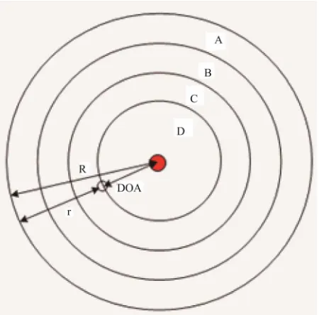
This paper proposes a new monitoring system model used to predict the next state of moving agent(s) in a closed space as in Figure 1 by fusing information from
multiple sensors of different types.
The area under surveillance is divided into four zones A, B, C and D shown in Figure 1 where each is only a
[image:2.595.312.537.85.307.2]ring with a width that is wide enough to be completely covered by the sonar sensor’s cone diameter. This sensor
Figure 1. Security monitoring system space with the red circle denotes the valuable asset.
could be mounted in the middle of the ceiling of each ring and rotating at a fixed scanning speed to provide a total number of agents at any given time in any zone [6,7]. As shown in Figure 2 the model also reads in data
from a grid of laser sensors [6,8,9] to capture agent speed. The following laser sensor network was assumed; four sensors in the X direction and another set of four laser sensors in the Y direction with each of them reporting the agent(s) speed in feet per second as in Figure 2.
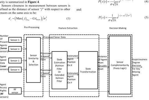
Finally an identification data transmitter is associated with each agent and captured by RF Radio Frequency sensor [10,11] to support the system with an ID of any moving agent. For sake of simplicity, Radio Frequency sensor will provide three pre-defined types of agent’s access rights (“Trusted”, “Semi-Trusted” and “Un-known”). Laser and sonar sensor data sets will then be fed into a sensor similarity processing sub-system that will be responsible to filter out any noisy sensor input of
X‐Direction
X‐Speed feet/sec Y‐Speed feet/sec
[image:2.595.309.536.575.721.2]each sensor-type and come up with a single reading based on sensor similarity method. After sensor data have been filtered, speed on X-axis and Y-axis outputs will be processed in a state estimation and transforma-tion.
where GAmean is the Global mean of all sensors (on a
given axis) and Max(j)Pos is the best estimate of the true
state of sensor “j” for data collected over one second time span sensor readings that are closest to the true state and defined as:
[image:3.595.62.541.397.720.2]Finally sensor complementarity stage starts where sensor data fusion/complementarity is performed using type-2 fuzzy logic inference system to produce a suspi-ciousness decision for each moving agent as shown in
Figure 3.
Max j Pos Max Posteriori xj (2)
where Posteriori of jth sensor’s reading given the
obser-vation xj is P(sj|xj).
4.1. Iterative Bayes Estimate and Maximum Posteriori
4. System Framework (Sensor Similarity)
Considering raw sensor measurements into sensor fusion may affect quality of fusion which leads to making wrong decisions in some cases where these measure-ments contain noisy and inaccurate data. Therefore, pre- processing of this sensory data plays an important role in sensor fusion. Only reliable subsets of the sensors are needed; subsets that are consistent and accurate.In this estimate the posterior of the different sensors was obtained based on Bayes formula:
P x s P s
P s x
P x
(3)
where “s” is the state and “x” is the observation. The probability of “s” given the observation “x”; the observa-tion drawn from normal distribuobserva-tion N(µ,σ2) where µ is the mean and σ standard deviation, so the mean of the likelihood function is the state under consideration which is represented as:
In our proposed system data is collected from a total of eight different laser sensors mounted on the X-axis and on the Y-axis (four sensors on each axis) with each sen-sor having different standard deviation and mean. This paper proposes a new method of sensor similarity that utilizes the concepts of relative closeness of sensors with respect to each other. Over all logic flow of sensor
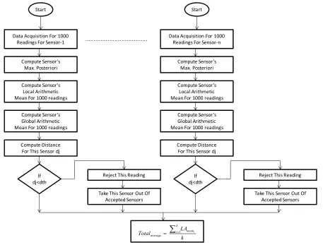
simi-larity is summarized in Figure 4.
2 2 2
1 2
x s
P x s e
(4)
Sensors closeness in measurement between sensors is defined as the distance of sensor “j” with respect to other
sensors on the same axis to be: and:
1
2 2 2
2
x
P x e
(5)
Max
2j Pos mean j
d j GA (1)
Sensor Similarity & Selection State Estimation (Kalman Filter Or Extended Kalman Filter State Transformation Sensor Complementarity
(Fuzzy Logic) Sensor‐1
Sensor‐n
Sensor‐1
Sensor‐n
RF sensor Number Of Present Agents (Sonar sensors) Agent Speed Data (Laser sensors) Agent Access Rights (RF sensors) Processed X‐Speed Data
Processed Y‐Speed Data
Processed Sonar Data
Estimated Agent Position On X
Estimated Agent Position On Y
Distance Of Agent From Valuable Asset Suspiciousness Degree Decision For Any Moving Agent
Pre‐Processing Feature Extraction Decision Making
Figure
4
Data Acquisition For 1000 Readings For Sensor‐1
Compute Sensor’s Max. Posteriori
Start
Compute Sensor’s Local Arithmetic Mean For 1000 readings
Compute Sensor’s Global Arithmetic Mean For 1000 readings
Compute Distance For This Sensor dj
If dj<dth
Reject This Reading
Take This Sensor Out Of
Accepted Sensors
1 k meani i average LA k Total
Data Acquisition For 1000 Readings For Sensor‐n
Compute Sensor’s Max. Posteriori
Start
Compute Sensor’s Local Arithmetic Mean For 1000 readings
Compute Sensor’s Global Arithmetic Mean For 1000 readings
Compute Distance For This Sensor dj
If dj<dth
Reject This Reading
Take This Sensor Out Of
Accepted Sensors
1 i k mean i average LA k
[image:4.595.73.530.85.432.2]Total
Figure 4. Flow chart shows how sensor similarity is performed.
The only unknown term left in Bayes is P(x). We know that:
1P s x
(6) so:
1P x s P s
P x
(7)then:
P x
P x s P s (8)The right side of Equation (8) is computed for all ob-servations and then divided by the total sum of these val-ues to compute P(x|s). This process was made iterative as more observations arrive by setting the priori Pr(i + 1)=
Posteriori of the previous observation P0(i) and the maximum posteriori is pulled out at each iteration.
4.2. Global and Local Means
In this paper, the LAmean is defined to be the Local Mean [12] for each sensor over its k observations and defined
mean
1
1 k i
i
LA k x
(9)and GAmean in Equation (1) to be the mean of all sensor local means that is defined as follows:
4 mean 1 mean n LA GA n
(10)where n is the number of used sensors for an axis (n = 4 in our example) and finally, σ in Equation (1) refers to the standard deviation of the sensor “j” given the fact that each sensor has a different mean and standard deviation.
After each sensor’s dj is calculated it is compared to a
pre-defined threshold distance dth to determine if the
reading of this sensor should be rejected or considered. In this paper we assume threshold dthis concluded from a
previously conducted calibration of the sensor network. If the sensor’s reading is considered then it is factored in when calculating the overall average of all considered readings: mean 1 average Total i n i LA n
[image:4.595.55.289.485.597.2]where “n” here is the total number of accepted sensors. Finally, a single reading as a similarity output is ob-tained. This algorithm of similarity is applied to laser sensors on both X axis and Y axis, and to the sonar sen-sors as well.
5. State Estimation and Transformation
5.1. Extended Kalman Filter
Real life dynamic systems and sensors are not absolutely linear, but they are close to be. Thus, applying Extended Kalman filter (EKF) on non-linear problems is a better fit.
Extended Kalman filtering is a method that linearizes about the covariance and current mean [13,14].
Extended Kalman filter uses measurements that are observed over time that contain noise, and produces val-ues that tend to be closer to the true valval-ues of the meas-urements and their associated calculated values. The Ex-tended Kalman filter is a set of mathematical equations that provides an efficient computational (recursive) means to estimate the state of a process, in a way that minimizes the mean of the squared error. Extended Kalman filtering is an ongoing cycle of time updating that projects the current state estimate ahead in time and the measurement updating that adjusts the projected estimate by an actual measurement at that time. The equations for those two updates are presented below [13,14]:
The first step is the Prediction (EKF time update): 1-Project the state ahead:
1,k k k
X f X u (12)
where Xk is the state vector (agent’s position and
veloc-ity), Ak is the state transition model that is applied to the
previous state Xk–1, Bk is the control input model that is
applied to the control vector uk and wk is the process
noise that is assumed to be drawn from a zero mean normal distribution with covariance Q.
1,k k k
X f X u (13)
2-Project the error covariance ahead:
1 T
k k
PAP A Q
(14) The second step is the update (EKF measurement up-date):
1-Compute the EKF gain:
1T T
k k k
K P H HP H R
k
(15)
where H is the measurement vector of the measurement zk of the true state space:
k k
z h x v (16) vkis the measurement noise that is assumed to be drawn
from a zero mean normal distribution with covariance R. 2-Update estimate with measurement zk:
k k k k k
x xK z h x (17)
3-Update the error covariance:
k k
P I K H P
k (18)
For application purposes, estimates of the agent’s po-sition on the X and the Y axes of the space are needed. Extended Kalman Filter was chosen to accomplish this task.
A system state was defined in this case to be the posi-tion and the speed.
average _ Total
x
V X (19)
average _ Total
y
V Y (20)
where the agent’s speed at the X-axis is the final
average
Total that was arrived at. After collecting agent’s data on X axis and deriving its corresponding position data as (same applies for the Y axis):
X
average
Total
x
P t X (21)
average
Total
y
P t Y (22)
where, t is the time.
Extended Kalman filter was applied on our system to estimate agent’s next position.
5.2. State Transformation (Homogeneous Sensor Complementarity)
Multi-sensor complementarity is the synergistic use of the information provided by different sensory devices to assist in the accomplishment of a system task. It refers to any stage in the integration process where there is an actual combination of different sources of sensory infor-mation into one sensory representation [15]. Sensor complementarities or correlation is especially advanta-geous when heterogeneous sensors are employed because of the potential to aggregate different views of the same incident.
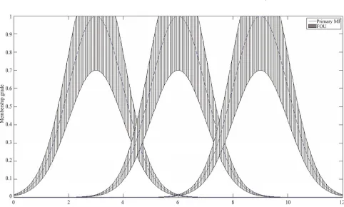
cal-It is the bounded area in Figure 5 and mathematically
it is the union of the upper and lower membership func-tions [14,18], where the upper and lower memberships are Gaussian functions:
culated to be R−r; where R is the radius of the largest circle where the agent is first detected by the sensors (Figure 1).
6. Decision Making/Type-2 Fuzzy
(Hetrogeneous Sensor Complementarity)
Upper
FOU A
N m
,2;x
(25)
1
Lower FOU A N m, ; x (26) The last part of this proposed system is the security
deci-sion making which utilizes the previous sub-system out-put to make a decision using an interval type-2 fuzzy system since it is suitable to make a precise decision in uncertain circumstances.
where, σ1 and σ2 are the standard deviations for lower and upper membership functions respectively and m is the mean of both.
6.2. Heterogeneous Sensor Complementarity 6.1. Interval Type-2 Fuzzy Inference System
Unlike a type-1 set where the membership grade is a crisp value in [0, 1], a type-2 fuzzy set shown in Figure 5 is characterized by a fuzzy membership function, where
the membership of each point of this set is a fuzzy set in [0, 1] [16].
An Interval type-2 fuzzy set makes room for non-de-terministic truth degree and uncertainty [17,18] (foot print of uncertainty FOU shown in Figure 5) for an
ele-ment that belongs to a set. A type-2 fuzzy set denoted by, à is characterized by a type-2 membership function, µÃ(x, u), where x X , u
0,1x
u J and 0 ≤µÃ(x, u) ≤ 1.
A
x,A
x
x X
(23)
, ,
,
, u
0,1
x A
A x u x u x X u J (24)
[image:6.595.58.540.432.722.2]f
DoA DoA f (27)
where (DoA) “Distance of Agent” from the asset in feet. DoA is categorized into four different fuzzy categories, “Agent is extremely close”, “Agent is very close”, “Agent is close” and “Agent is far” (Figure 1). Also,
where “f” is a multiplication factor that is based on the “Access Rights” of any moving agent and defined to be twenty for a “Trusted” (denoted by “T”), ten for “Semi- Trusted” (denoted by “ST”) and finally a one for an “Un- known” agent (denoted by “U”).
The proposed system has only one output which is the “Degree of suspiciousness” (DoS). This DoS is catego-rized into five levels of suspiciousness, “Not suspicious”, “Almost Suspicious”, “Suspicious”, “Very Suspicious”, and “Extremely suspicious” as shown in Figure 6 and is
driven by the DoAf and NoA inputs [6,20].
7. Experimantal Results and Discussions
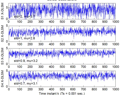
In this study a real-life simulation of several situations of agents moving non-linearly were investigated. Evalua-tion for a one agent is shown here. Assuming agent’s true speed is 3 feet/sec on X-axis the grid of four sensors (each sensor is slightly different from the other in its mean and standard deviation) captured this speed over one second time frame. Figure 7 shows agent speedcap-tured by four sensors.
Sensor 1 of this group is assumed to be noisier with mean and standard deviation well distant from the other three. We also assumed the agent’s true speed is 5 feet/sec on Y-axis, the grid of four sensors (each sensor is slightly different from the other in its mean and stan-dard deviation) on this axis also captured this speed over same time interval that is 1 second Figure 8 shows this
agent’s data on the Y-axis. Sensor 2 of this group is as-sumed to be the noisy sensor.
[image:7.595.307.539.91.275.2]Figure 6. System suspiciousness levels.
[image:7.595.307.540.343.532.2]Figure 7. Speed data read by four laser sensors on the X-axis of the sensor grid (where DLSM is Direction Laser Speed Measurement) and the number prefix refers to the sensor index in the grid.
Figure 8. Speed data read by four laser sensors on the X-axis of the sensor grid (where DLSM is Direction Laser Speed Measurement) and the number prefix refers to the sensor index in the grid.
Local means were next computed for each the four sensors on X-axis over for measurement over one second are shown in Figures 9 and 10 show their equivalents on
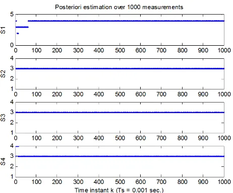
the Y-axis for the same time span. The next step in our sensor similarity is to compute the maximum posteriori for each of the X-axis sensors which are displayed in
Figure 11 and compute those posteriori for the Y-axis as
well as shown in Figure 12. After sensor similarity is
[image:7.595.58.289.529.718.2]Figure 9. Local mean (LAmean) for the four sensors on the
X-axis over 1 second time span.
[image:8.595.307.540.84.274.2]Figure 11. Max. posteriori (Max(j)pos) for the four sensors on the X-axis over 1 second time span.
Figure 10. Local mean (LAmean) for the four sensors on the
Y-axis over 1 second time span.
Figure 12. Max. posteriori (Max(j)pos) for the four sensors on the Y-axis over 1 second time span.
Those thresholds are assumed to be based on sensor calibration data for each axis. New global mean (Total av-erage) was computed but based on only accepted sensors. Next Extended Kalman filter was used to estimate agent’s next state (next accumulated distance) on both axes based on the X-Totalaverage and Y-Totalaverage that are shown in Figures 13 and 14 respectively.
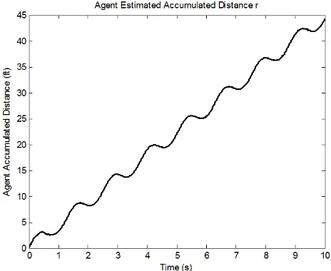
State estimation (S.T.) that is the second to last block in our security system is then utilized to transform the distance data on (x, y) coordinates to (r,θ) polar coordi-nates (homogeneous sensor complementarity) as in Fig-ure 15.
Finally, a weighing is applied to this computed r (based on its access right that is chosen to be 1.3 and 1.1 for “Trusted” and “Semi-Trusted” respectively and 1 for “Un-
decide on its suspiciousness degree at any time during its movement shown in Figure 16. This figure displays eva-
luation two agents having the same speed values but dif-ferent access rights (“Trusted” and “Unknown”). Figure 16 shows how the proposed security system was able to
limit the DoS for the “Trusted” agent to less than 55%. However, it gave the “Unknown” agent almost a 65% for the same speed and distance accumulated values. It was shown that our system can actually use normal sensor data to filter it, estimate state, transform state and make a decision.
8. Conclusions and Future Work
[image:8.595.57.288.311.503.2] [image:8.595.308.538.311.499.2]Figure 13. Agent position on X axis where “0” is the point where agent was first detected by the sensor.
[image:9.595.55.287.314.504.2]Figure 15. Agent accumulated distance in polar coordinates.
Figure 14. Agent position on Y axis where “0” is the point where agent was first detected by the sensor.
Figure 16. Agent suspiciousness degree as it moves.
security monitoring system. With the Extended Kalman filter and interval type-2 fuzzy inference help, the system was further able to estimate agent’s next state and report its security status. The proposed system exhibits promis-ing performance in security awareness systems and agent security status evaluation accounting for dynamics, non-linearity and uncertainty.
One planned future system improvement is to intro-duce active relationship between multiple agents and environment.
9. Acknowledgements
Authors would like to thank Prof. O. Castillo for provid-ing us his own made type-2 fuzzy toolbox [19], his help is much appreciated.
REFERENCES
[1] M. Zohdy and A. Khan, “Global Optimization of Sto-chastic Multivariable Functions,” American Control Con-
ference, San Francisco, 2-4 June 1993, p. 2339.
[2] H. Hujun and Z. Yaning, “Multi-Source Data Fusion Technology and Its Application in Geological and Min-eral Survey,” 2010 2nd International Conference on
In-formation Engineering and Computer Science (ICIECS),
Wuhan, 25-26 December 2010, pp. 1-6.
[3] D. L. Hall and J. Llinas, “An Introduction to Multisensor Data Fusion,” Proceedings of the 1998 IEEE
Interna-tional Symposium on Circuits and Systems, 31 May-3
June 1998, pp. 537-540.
[4] Q. Wu, D. Ferebee, Y. Lin and D. Dasgupta, “An Inte-grated Cyber Security Monitoring System Using Correla-tion-Based Techniques,” IEEE International Conference
[image:9.595.308.538.315.502.2]May-3 June 2009, pp. 1-6.
[5] R. Tenney and N. Sandell, “Detection with Distributed Sensors,” IEEE Transactions on Aerospace and
Elec-tronic Systems, Vol. AES-17, No. 4, 1981, pp. 501-510.
[6] T. Dakhlallah, M. Zohdy and O. Salim, “Application of Hyper-Fuzzy Logic Decisions for A Security Monitoring System,” 2011 3rd International Conference on
Com-puter and Automation Engineering (ICCAE 2011), 2011,
p. V1-387.
[7] LV-MaxSonar-EZ0, “High Performance Sonar Range Finder,” MaxBotix Inc., 2005.
[8] CSI 430, “SpeedVueTM Laser Speed Sensor,” Emerson Process Management, 2009.
[9] MiniVLS nL, “Series Optical Speed/Phase Sensors VLS nL,” Compact Instruments.
[10] Tag-it HF-I Standard, 13.56 MHz, “Transponder Inlays, ISO/IEC 15693 and ISO/IEC 18000-3 Global Open Stan-dards,” Texas Instruments, 2005.
[11] Smart Card SCC-3, “3.125KHz+UHF EPC GEN2,” Rui Yue RFID Co., 2006.
[12] Albert Leon-Garcia, “Probability and Random Processes for Electrical Engineering,” 2nd Edition, Pearson/Prentice Hall, Upper Saddle River, 2008.
[13] G. Welch and G. Bishop, “An Introduction to the Kalman Filter,” University of North Carolina at Chapel Hill, Chapel Hill, 2001.
[14] E. Ayachi, S. Ihsen and B. Mohamed, “A Comparative
Study of Nonlinear Time-Varying Process Modeling Techniques: Application to Chemical Reactor,” Journal
of Intelligent Learning Systems and Applications,Vol. 4,
No. 1, 2012, pp. 20-28.
[15] R. C. Luo and C. Yih, “Multisensor Fusion and Integra-tion: Approaches, Applications and Future Research Di-rectories,” IEEE Sensors Journal, Vol. 2, No. 2, 2002, pp. 107-119.
[16] O. Castilo and P. Mellin, “Type-2 Fuzzy Logic: Theory and Applications,” Tijuana Institute of Technology,
Divi-sion of Graduate Studies, Vol. 223, 2008.
[17] Q. Liang and J. Mendel, “Interval Type-2 Fuzzy Logic Systems: Theory and Design,” IEEE Transactions on
Fuzzy Systems, Vol. 8, No. 5, 2000, pp. 535-550.
[18] J. Mendel, “Uncertain Rule-based fuzzy logic systems: Introduction and New Directions,” Prentice-Hall, Upper Saddle River, 2001.
[19] H. Youpeng, L. Lin and Z. Yongfeng, “A Hetrogenous Sensors Track-to-Track Correlation Algorithm Based on Fuzzy Numbers Similarity Degree,” Second International
Conference on Information and Computing Science,2009
Manchester, 21-22 May 2009, pp. 191-194.
[20] J. R. Castro, O. Castillo and P. Melin, “An Interval Type-2 Fuzzy Logic Toolbox for Control Applications,”
International Conference on Fuzzy Systems, London,
23-26 July 2007, pp. 1-6.