A Semi Supervised Deep Rule Based Approach for Remote Sensing Scene Classication

for Remote Sensing Scene Classification

Xiaowei Gu1,2[0000−0001−9116−4761] _{and Plamen P.} Angelov1,2,3,∗[0000−0002−5770−934X]

1

School of Computing and Communications, Lancaster University, LA1 4WA, UK

2

Lancaster Intelligent, Robotic and Autonomous Systems Centre (LIRA), Lancaster University, UK

3

Honorary Professor, Technical University, Sofia, 1000, Bulgaria * Corresponding Author

p.angelov@lancaster.ac.uk

Abstract. This paper proposes a new approach that is based on the recently introduced semi-supervised deep rule-based classifier for remote sensing scene classification. The proposed approach employs a pre-trained deep convoluational neural network as the feature descriptor to extract high-level discriminative semantic features from the sub-regions of the remote sensing images. This approach is able to self-organize a set of prototype-based IF...THEN rules from few labeled training images through an efficient supervised initialization process, and continuously self-updates the rule base with the unlabeled images in an unsupervised, autonomous, transparent and human-interpretable manner. Highly accurate classifi-cation on the unlabeled images is performed at the end of the learning process. Numerical examples demonstrate that the proposed approach is a strong alternative to the state-of-the-art ones.

Keywords: Deep rule-based·Remote sensing scene classification· Semi-supervised learning.

1

Introduction

networks (DCNNs) require a large amount of labeled images for training [6,9,12]. In reality, labeled remote sensing images are scarce and expensive to obtain, but unlabeled images are plentiful. Supervised approaches, however, are unable to use the unlabeled images. On the other hand, semi-supervised machine learning approaches [13–16] consider both the labeled and unlabeled images for classifica-tion, and, thus, they are able to utilize information from the unlabeled images to a greater extent. Nonetheless, there are only very few published works applying semi-supervised techniques to remote sensing scene classification [17–19]. Semi-supervised deep rule-based (SSDRB) approach [20] is introduced as an semi-supervised learning extension of the deep rule-based (DRB) approach [11, 21] for image classification. In comparison with alternative approaches [13– 19], the SSDRB classifier is able to perform semi-supervised learning in a self-organizing, fully transparent and human-interpretable manner thanks to its prototype-based nature. By exploiting the idea of “pseudo labeling”, the SS-DRB classifier can learn from unlabeled images offline and identify new classes actively without human expertise involvement. It further supports online learn-ing on a sample-by-sample or chunk-by-chunk basis

In this paper, a new SSDRB-based approach is proposed for remote sensing scene classification. The proposed approach extends the idea of our previous works [11, 22] by conducting semi-supervised learning on the local regions of the remote sensing images. Using a DCNN-based feature descriptor [23] to extract high-level semantic features from the images locally, the SSDRB classifier is able to self-organize a set of prototype-based IF...THEN rules [24] from the local re-gions of, both, labeled and unlabeled images, and classify the unlabeled images based on the score of confidence obtained from each sub-region locally.

2

The Proposed Approach

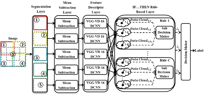
The general architecture of the SSDRB classifier used in this paper is given by Fig. 1. As one can see from this figure, the SSDRB classifier is composed of the following components:

1. segmentation layer; 2. mean subtraction layer; 3. feature descriptor layer; 4. IF...THEN rule-based layer; 5. decision-maker,

and, their functionalities are described in the following five subsections, respec-tively.

2.1 Segmentation Layer

Fig. 1: The general architecture of SSDRB classifier.

descriptor [23]. In comparison with using the whole image for classification, seg-menting the image in this way enables the feature descriptor to extract the semantic features locally, and, thus, improve the generalization ability of the proposed approach.

2.2 Mean Subtraction Layer

This layer pre-processes the segments by mean subtraction for feature extraction. This operation centers the three channels (R, G, B) of the segments around the zero mean, which helps the feature descriptor to perform faster since gradients act uniformly for each channel.

2.3 Feature Descriptor Layer

This layer is used for extracting high-level semantic feature vectors from the sub-regions of the images for the learning process. In this work, we use a pretrained VGG-VD-16 DCNN model [23] for feature extraction, and the 1×4096 dimen-sional activations from the first fully connected layer are used as the feature vector of each segment.

2.4 IF...THEN Rule-Based Layer

This layer is a massively parallel ensemble of zero-order IF...THEN rules of AnYa type, which is the “core” of the SSDRB classifier. The SSDRB classifier is, firstly, trained in a fully supervised manner with the labeled training set [20, 21]. As-suming that there are theC known classes based on the labeled remote sensing images, C IF...THEN rules are initialized in parallel from the segments of la-beled images of the corresponding classes (one rule per class).

continuously updated based on the segments of the unlabeled images in a self-organizing manner. The SSDRB classifier is also able to perform active learning without human interference [20], but, we only consider the semi-supervised learn-ing in this paper. Once the whole learnlearn-ing process is finished, one can obtain a set of IF...THEN rules in the following form [11, 20, 21] (c= 1,2,3, ..., C):

IF(s∼Pc,1)OR(s∼Pc,2)OR ...OR (s∼Pc,Nc)THEN (class c) (1) where “∼” denotes similarity, which can also be seen as a fuzzy degree of mem-bership;sis a segment of a particular image, andxis the corresponding feature vector extracted by the DCNN model; Pc,i stands for the ith visual prototype of thecth_{class, and p}

c,i is the corresponding feature vector;i= 1,2, ..., Nc;Nc is the number of identified prototypes from the segments of images of the cth

class.

2.5 Decision-Maker

During the validation process, for each segment of the unlabeled remote sensing images, theC IF...THEN rules will generate a vector of scores of confidence:

λ(sk,j) = [λ1(sk,j), λ2(sk,j), ..., λC(sk,j)] (2) wheresk,jdenotes thejth(j= 1,2,3,4, Ko;Ko= 5) segment of thekthunlabeled image,Ik;λc(sk,j) stands for the score of confidence given by thecthIF...THEN rule using the following equation:

λc(sk,j) = max i=1,2,...,Nc

(e−||xk,j−pc,i||2_{) (3)}

wherexk,j corresponds to the feature vector of the visual prototype,Pc,i. The label of the remote sensing image is decided based on the vectors of scores of confidence calculated from all the segments:

Label(Ik)←class c∗; c∗= argmax c=1,2,...,C

( 1

Ko Ko X

j=1

λc(sk,j)) (4)

Due to the limited space of this paper, we skip the details of the supervised and semi-supervised learning processes of the SSDRB classifier. The detailed de-scription of the algorithmic procedure can be found in [20] and Chapter 9 of the book [25]. One can download the open source software implemented on Matlab platform from the following web link with a detailed instruction provided in the Appendix C of the book [25]:

3

Numerical Examples

In this section, numerical examples based on benchmark problems in the remote sensing domain are presented to demonstrate the performance of the proposed approach.

3.1 Experimental Setup

In this paper, we consider the following widely used benchmark datasets: 1. Singapore dataset;

2. WHU-RS dataset; 3. RSSCN7 dataset.

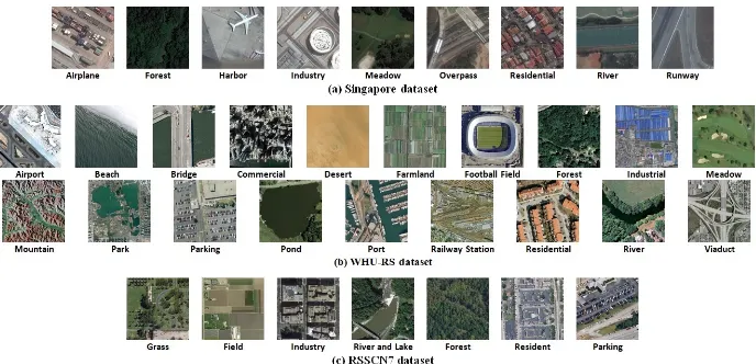
Singapore dataset [26] is a recently introduced benchmark image set for re-mote sensing scene classification. This image set consists of 1086 images of size 256×256 pixels with nine categories:i)airplane,ii)forest,iii)harbor,iv) indus-try, v) meadow, vi) overpass, vii) residential, viii) river, and ix) runway. This image set is imbalanced, and the number of images in each class varies from 42 to 179. Examples of images of the nine classes are given in Fig. 2(a).

Fig. 2: Example images of the benchmark datasets.

xiv)pond,xv)port,xvi)railway,xvii)residential,xviii)river, andxix)viaduct. There are very high variations within the images in terms of illumination, scale, resolution, etc., which makes this a difficult classification problem. Examples of images of this problem are given in Fig. 2(b).

RSSCN7 dataset [28] is a benchmark problem also collected from Google Earth. This image set is composed of images of seven different classes, which include i) grassland, ii) forest, iii) farmland, iv) parking lot,v) residential re-gion,vi)industrial region,vii) river and lake. Each class has 400 images of size 400×400 pixels. This dataset is a very challenging one due to the fact that the images of each class are sampled on four different scales (100 images per scale) with different imaging angles. Examples of images of this problem are given in Fig. 2(c).

In this paper, we use the offline semi-supervised learning strategy for the SS-DRB classifier, and the user-controlled parameter required, namely, Ω1, is set to Ω1 = 1.2. The reported experimental results are the average after five times Monte Carlo experiments. The images of the WHU-RS dataset have been re-scaled into the same size as the images of the RSSCN7 dataset, namely, 400×400 pixels, to avoid the loss of information during the segmentation operation. We further involve the following seven popular approaches for comparison:

1. Deep rule-based classifier (DRB) [21];

2. Support vector machine classifier with linear kernel function (SVM) [29]; 3. k-nearest neighbor classifier (kNN) [30];

4. AnchorGraphReg-based semi-supervised classifier with kernel weights (An-chorK) [16];

5. AnchorGraphReg-based semi-supervised classifier with Local Anchor Em-bedding weights (AnchorL) [16];

6. Greedy gradient Max-Cut based semi-supervised classifier (GGMC) [14]; 7. Laplacian SVM semi-supervised classifier (LapSVM) [15, 17].

In the following numerical examples, the value ofkfor kNN is set tok= 5. The user-controlled parameter of AnchorK and AnchorL, s (number of the closest anchors) is set tos= 3, and the iteration number of Local Anchor Embedding (LAE) for AnchorL,is set to 10 as suggested in [16]. GGMC uses the KNN graph with k = 5. LapSVM employs the one-versus-all strategy, and it uses a radial basis function kernel withσ= 10. The two user-controlled parametersγIandγA are set to 1 and 10−6, respectively; the number of neighbour,k, for computing the graph Laplacian is set to 15 as suggested in [15]. For the comparative algorithms, we follow the common practice by averaging the 1×4096 dimensional feature vectors of the five sub-regions to generate an overall image representation as the input feature vector [3].

3.2 Experimental Results on the Singapore Dataset

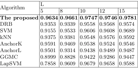
unlabeled ones to test the performance of the proposed approach. The classifi-cation accuracy on the unlabeled images obtained by the proposed approach is given in Table 1. We also report the results obtained by the seven comparative approaches in the same table.

Secondly, we follow the commonly used experimental protocol [26] by randomly selecting out 20% of images from each class as the labeled training images and using the remaining as the unlabeled ones, and report the classification perfor-mance of the eight approaches in Table 2. The state-of-the-art results reported by other approaches are also provided for a better comparison.

Table 1: Classification performance comparison on the Singapore dataset with different number of labeled training images.

Algorithm L

5 8 10 12 15

The proposed 0.9634 0.9661 0.9747 0.9746 0.9781

DRB 0.9353 0.9339 0.9558 0.9568 0.9574 SVM 0.9155 0.9533 0.9606 0.9608 0.9689 kNN 0.9375 0.9381 0.9548 0.9576 0.9592 AnchorK 0.9591 0.9469 0.9538 0.9524 0.9546 AnchorL 0.9501 0.9314 0.9438 0.9489 0.9487 GGMC 0.8999 0.8828 0.9422 0.9286 0.9447 LapSVM 0.7858 0.9609 0.9679 0.9658 0.9588

Table 2: Classification performance comparison on the Singapore dataset under the commonly used experimental protocol.

Algorithm Accuracy Algorithm Accuracy Algorithm Accuracy

The proposed 0.9793 DRB 0.9573 SVM 0.9643

kNN 0.9768 AnchorK 0.9678 AnchorL 0.9551

GGMC 0.9578 LapSVM 0.9293 TLFP [26] 0.9094 BoVW [31] 0.8741 VLAD [32] 0.8878 SPM [33] 0.8285

3.3 Experimental Results on the WHU-RS Dataset

Table 3: Classification performance comparison on the WHU-RS dataset under the commonly used experimental protocol.

Algorithm Accuracy Algorithm Accuracy Algorithm Accuracy

The proposed 0.9387 DRB 0.9228 SVM 0.9291

kNN 0.9235 AnchorK 0.9013 AnchorL 0.9126

GGMC 0.9073 LapSVM 0.9305 BoVW (SIFT) [7] 0.7526

VLAD (SIFT) [7] 0.7637 SPM (CH) [7] 0.5595 CaffeNet [7] 0.9511 VGG-VD-16 [7] 0.9544 GoogLeNet [7] 0.9312 salM3LBP-CLM [8] 0.9535

3.4 Experimental Results on the RSSCN7 Dataset

As a common practice [7], we randomly pick out 20% of images from each class, namely, 80 images per class as the labeled training images and use the remaining as the unlabeled ones, and conduct the experiments with the eight approaches. The experimental results are tabulated in Table 4. Similarly, the selected state-of-the-art results produced by other approaches are also reported in the same table.

Table 4: Classification performance comparison on the RSSCN7 dataset under the commonly used experimental protocol.

Algorithm Accuracy Algorithm Accuracy Algorithm Accuracy

The proposed 0.8670 DRB 0.8422 SVM 0.8529

kNN 0.8532 AnchorK 0.8413 AnchorL 0.8465

GGMC 0.7705 LapSVM 0.8398 BoVW (SIFT) [7] 0.7633

VLAD (SIFT) [7] 0.7727 SPM (CH) [7] 0.6862 CaffeNet [7] 0.8557 VGG-VD-16 [7] 0.8398 GoogLeNet [7] 0.8255 DBNFS [28] 0.7119

3.5 Discussion

Tables 1-4 demonstrate that the proposed SSDRB approach consistently out-performs the seven comparative approaches. The accuracy of the classification results it produced is above or at least at the same level with the state-of-the-art approaches. In addition, our previous works [20] also show that the SSDRB classifier can achieve very high performance even with only one single labeled image per class, and is able to learn new classes actively without human exper-tise involvement.

4

Conclusion

In this paper, a semi-supervised deep rule-based (SSDRB) approach is proposed for remote sensing scene classification. By extracting the high-level features from the sub-regions of the images, the proposed approach is capable of capturing more discriminative semantic features from the images locally. After the su-pervised initialization process, the proposed approach self-organizes its system structure and self-updates its meta-parameters from the unlabeled images in a fully autonomous, unsupervised manner. Numerical examples on benchmark datasets demonstrate that the proposed approach can produce state-of-the-art classification results on the unlabeled remote sensing images surpassing the pub-lished alternatives.

References

1. Sheng, G., Yang, W., Xu, T., et al.: High-resolution satellite scene classification using a sparse coding based multiple feature combination. Int. J. Remote Sens.

33(8), 2395–2412 (2012)

2. Cheriyadat, A. M.: Unsupervised feature learning for aerial scene classification. IEEE Trans. Geosci. Remote Sens.52(1), 439–451 (2014)

3. Hu, F., Xia, G.-S., Hu, J., et al.: Transferring deep convolutional neural networks for the scene classification of high-resolution remote sensing imagery. Remote Sens.

7(11), 14680–14707 (2015)

4. Chen, S., Tian, Y.: Pyramid of spatial relatons for scene-level land use classification. IEEE Trans. Geosci. Remote Sens.53(4), 1947–1957 (2015)

5. Zhang, L., Zhang, L., Kumar, V.: Deep learning for remote sensing data. IEEE Geosci. Remote Sens. Mag.4(2), 22–40 (2016)

6. Scott, G.-J., England, M. R., Starms, W. A., et al.: Training deep convolutional neu-ral networks for land-cover classification of high-resolution imagery. IEEE Geosci. Remote Sens. Lett.14(4),549–553 (2017)

7. Xia, G.-S., Hu, J., Hu, F., et al.: AID: a benchmark dataset for performance evalu-ation of aerial scene classificevalu-ation. IEEE Trans. Geosci. Remote Sens.55(7), 3965– 3981 (2017)

8. Bian, X., Chen,C., Tian, L., et al.: Fusing local and global features for high-resolution scene classification. IEEE J. Sel. Top. Appl. Earth Obs. Remote Sens.

10(6), 2889–2901 (2017)

9. Li, Y., Zhang, H., Shen, Q.: Spectral-spatial classification of hyperspectral imagery with 3D convolutional neural network. Remote Sens.9(1), 67 (2017)

10. Liu, R., Bian, X., Sheng, Y.: Remote sensing image scene classification via multi-feature fusion. In: Chinese Control and Decision Conference, 3495–3500 (2018) 11. Gu, X., Angelov, P., Zhang, C., et al.: A massively parallel deep rule-based

ensem-ble classifier for remote sensing scenes. IEEE Geosci. Remote Sens. Lett.32(11),345– 349 (2018)

12. Zhang, M., Li, W., Du, Q., et al.: Feature extraction for classification of hyper-spectral and LiDAR data using patch-to-patch CNN. IEEE Trans. Cybern. (2018). https://doi.org/10.1109/TCYB.2018.2864670

14. Wang, J., Jebara, T., Chang, S.-F.: Semi-supervised learning using greedy Max-Cut. J. Mach. Learn. Res.14771–800 (2013)

15. Belkin, M., Niyogi, P., Sindhwani, V.: Manifold regularization: a geometric frame-work for learning from labeled and unlabeled examples. J. Mach. Learn. Res. 7

2399–2434 (2006)

16. Liu, W., He, J., Chang, S.-F.: Large graph construction for scalable semi-supervised learning. In: International Conference on Machine Learning, 679–689 (2010) 17. Gmez-Chova, L., Camps-Valls, G., Munoz-Mari, J., et al.: Semisupervised image

classification with Laplacian support vector machines. IEEE Geosci. Remote Sens. Lett.5(3) 336–340 (2008)

18. Bruzzone, L., Chi, M., Marconcini, M.,: A novel transductive SVM for semisu-pervised classification of remote-sensing images. IEEE Trans. Geosci. Remote Sens.

44(11) 3363–3373 (2006)

19. Huo, L., Zhao, L., Tang, P.,:Semi-supervised deep rule-based approach for image classification. In: Workshop on Hyperspectral Image and Signal Processing: Evolu-tion in Remote Sensing (WHISPERS), 1–4 (2014)

20. Gu, X., Angelov, P.: Semi-supervised deep rule-based approach for image classifi-cation. Appl. Soft Comput.6853–68 (2018)

21. Angelov, P., Gu, X.: Deep rule-based classifier with human-level performance and characteristics. Inf. Sci. (Ny).463-464196–213 (2018)

22. Gu, X., Angelov, P.: A deep rule-based approach for satellite scene image analysis. In: IEEE International Conference on Systems, Man and Cybernetics (2018) 23. Simonyan, K., Zisserman, A.: Very deep convolutional networks for large-scale

image recognition. In: International Conference on Learning Representations 1–14 (2015)

24. Angelov, P., Yager, P.,: A new type of simplified fuzzy rule-based system. Int. J. Gen. Syst.41(2) 163–185 (2011)

25. Angelov, P., Gu, X.: Empirical approach to machine learning. Springer Interna-tional Publishing (2019)

26. Gan, J., Li, Q., Zhang, Z., et al.: Two-level feature representation for aerial scene classification. IEEE Geosci. Remote Sens. Lett.13(11) 1626–1639 (2016)

27. Xia, G., Yang, W., Delon. J., et al.: Structural High-resolution Satellite image in-dexing. In: ISPRS, TC VII Symposium Part A: 100 Years ISPRSAdvancing Remote Sensing Science 298–303 (2010)

28. Zou, Q., Ni, L., Zhang, T., et al.: Deep learning based feature selection for remote sensing scene classification. IEEE Geosci. Remote Sens. Lett. 12(11) 2321–2325 (2015)

29. Cristianin, N., Shawe-Taylo, J.: An introduction to support vector machines and other kernel-based learning methods. Cambridge University Press, Cambridge (2000)

30. Cunningham, P., Delany, S.-J.: K-nearest neighbour classifiers. Mult. Classif. Syst.

34(11) 1–17 (2017)

31. Yang, Y., Newsam, S.: Bag-of-visual-words and spatial extensions for land-use classification. In: International Conference on Advances in Geographic Information Systems 270–279 (2010)

32. Jgou, H., Douze, M., Schmid, C.: Aggregating local descriptors into a compact representation. In: IEEE Conf. Comput. Vis. Pattern Recognit. 3304–3311 (2010) 33. Lazebnik, S., Schmid, C., Ponce, J.,: Beyond bags of features: spatial pyramid