A Bayesian Hierarchical Model For Longitudinal Data

(1)

RESEARCH ARTICLE

A BAYESIAN HIERARCHICAL MODEL FOR LONGITUDINAL DATA

Senthamaraikannan, K2_{Senthilkumar, B}

1

_{Tuberculosis Research Centre, Indian Council of Medical Research, Chennai}

2

_{Manonmaniam Sundaranar University, Tirunelveli}

ARTICLE INFO ABSTRACT

The paper investigates a Bayesian hierarchical model for the analysis of longitudinal data from a randomized controlled clinical tuberculosis trial. Data for each subject are observed on thirteen time point of occasions of the trial. One of the features of the data set is that observations for some variables are missing for at least one time point. In the Bayesian approach, to estimate the model, we use th

the response and the explanatory variables to impute at each iteration of the algorithm, given some appropriate prior distributions.

INTRODUCTION

Bayesian methods are based on the assumption that probability is operationalized as a degree of belief, and not a frequency as is done in classical, or frequentist, statistics. Most researchers in marketing have been trained to think about statistics in terms of frequencies. Serious investigation of biological processes is challenging due to the complex nature of these processes and the lack of sufficient data and missing. Hence, compromised to turn to stochastic modeling as a means to capture the uncertainty in our inference about the process. In view of the fact that typically, such processes involve components at different stages and time points, it is natural to frame our modeling in the context of hierarchical models. Since such models introduce unknowns and it is needed to incorporate the uncertainty associated

*Corresponding author:cponnuraja@gmail.com

with these unknowns in order to achieve a better overall assessment of the uncertainty in our modeling. This promotes us to convey the models under the Bayesian framework. The objective of this paper is to provide an introduction as we an application to the tools to work with Bayesian hierarchical modeling with randomized controlled clinical trial data.

MCMC ALGORITHM

The most commonly used algorithm in MCMC applications are two types and they are Metropolis Algorithms and Gibbs sampler. Geman and Geman (1984) presented the Gibbs sampler in context of spatial processes involving large number of variables like image reconstructions. They consider under which s

given neighborhood subsets of the variables, which they uniquely determines the joint distribution. Basic contribution as the framework of iterative

ISSN: 0975-833X

International Journal of Current Research Vol.10, pp.012-020, November

Key words:

Bayesian hierarchical model, Longitudinal data, Gibbs sampler

Article History:

Received 8th_{September, 2010}

Received in revised form 17th_{October, 2010}

Accepted 25th October, 2010 Published online 1st_{November, 2010}

ARTICLE

A BAYESIAN HIERARCHICAL MODEL FOR LONGITUDINAL DATA

B2_{Ponnuraja, C}1_{and Venkatesan, P}1

Tuberculosis Research Centre, Indian Council of Medical Research, Chennai-31

Sundaranar University, Tirunelveli-627012

ABSTRACT

The paper investigates a Bayesian hierarchical model for the analysis of longitudinal data from a randomized controlled clinical tuberculosis trial. Data for each subject are observed on thirteen time point of occasions of the trial. One of the features of the data set is that observations for some variables are missing for at least one time point. In the Bayesian approach, to estimate the model, we use the Gibbs sampler, which as well allows missing data for both the response and the explanatory variables to impute at each iteration of the algorithm, given some appropriate prior distributions.

with these unknowns in order to achieve a better overall assessment of the uncertainty in our modeling. This promotes us to convey the models under the Bayesian framework. The objective of this paper is to provide an introduction as well as an application to the tools to work with Bayesian hierarchical modeling with randomized controlled clinical trial data.

MCMC ALGORITHM

The most commonly used algorithm in MCMC applications are two types and they are Metropolis Algorithms and Gibbs sampler. Geman and Geman (1984) presented the Gibbs sampler in context of spatial processes involving large number of variables like image reconstructions. They consider under which situations the conditional distributions given neighborhood subsets of the variables, which they uniquely determines the joint distribution. Basic contribution as the framework of iterative

ternational Journal of Current Research 020, November, 2010

INTERNATIONAL JOURNAL OF CURRENT RESEARCH

(2)

Monte Carlo algorithms performed by Tanner and Wang (1987). Further developments in the fields listed here the data augmentation by Gelfand and Smith (1990), Gibbs sampler and the sampling important resampling (SIR) algorithm by Rubin (1987). The applications of the Gibbs sampler to mixture of important statistical problem were discussed by many researchers correspondingly Gelfand et al(1990), Gelfand and Smith (1991), Carlin and Polson (1991), Carlin et al. (1992), Gelfand et al (1992). The Metropolis-Hastings algorithm was developed by Metropolis, et al., (1953) and consequently generalized by Hastings (1970). A broad theoretical description of Metropolis-Hastings was given by (Tierney, 1994; Chib and Greenberg, 1995) provide an outstanding discussion.

Using Metropolis Algorithm to construct a Markov chain with equilibrium distribution 

 

x for discrete case, Let Q

 

q_ij be specified symmetric

transition matrix and draw state

s

_jfrom ith of row

of

Q

. With known probability



_ij move from the

state

s

_i to the state

s

_j, otherwise, remain at step

s

_i

. The construction defines a Markov chain with

transition matrix _p _q _i _j

ij ij

ij   and





 

i j ij

ij p

p 1 . Metropolis et al (1953), we let

    

  

1 / ,

/

1 / ,

1

i j i

j

i j ij

if if

  



 

 [1]

Gibbs sampler and Metropolis-Hastings algorithm

The Gibbs sampler technique is one of the best known MCMC sampling algorithms in the Bayesian computational methods. The Gibbs sampler established by Besag and Green (1993) and the ideas of Grenander (1983), the prescribed term is introduced by Geman and Geman (1984). Gibbs sampling is the landmark in problem of Bayesian inference (Gelfand and Smith, 1990). The Gibbs sampler tutorial is provided by Casella and George (1992).

Let









₁

,



₂

,...,



_p



' be a p-dimensional vector

of parameters and let







|

D



be its posterior distribution given the data D. Then, the fundamental format of the Gibbs sampler is given as

Step1. Select an arbitrary starting point



₁₀ ₂₀ ₀



0

0  , ,..., and set i

' , p , ,



Step 2. Generate_i_₁ 



₁_,_i_₁,₂_,_i_₁,...,_p_,_i_₁



'

Generate 1_,_i1~



1|2_,_i,...,_p_,_i,D



;

Generate



2_,_i1

~







2

|



1_,_i1

,



3_,_i

,...,



_p_,_i

,

D



;

… … …

Generate



p,i1~







p|



1,i1,



2,i1,...,



p1,i1,D



;

Step 3. Set

i



i



1

, and go to step 2

Each component of θ is in the natural order and a cycle in this scheme requires generation of p random variates. Gelfand and Smith (1990) show that under certain regularity conditions, the vector sequence

   

 

 , ,... i ,

i 12

 has a stationary distribution



|D



 . Schervish and Carlin (1992) provide a sufficient condition that guarantees geometric convergence and all other properties of geometric convergence are discussed by Roberts and Polson (1994).

Metropolis-Hastings

Let

q





,





be a proposal density, which is also termed as a candidate generating density by Chib and Greenberg (1995),

_

_q

_

__,_

_

_d__₁ also let

U(0,1) denote the uniform distribution over (0,1), Then, a general version of the Metropolis-Hastings algorithm for sampling from the posterior distribution







|D



can be described as

Step1. Select an arbitrary starting point



₀ and set i=0

Step 2. Generate a candidate point



*from

 

.

(3)

Step 3. Set



*



_i _i i

*

i  if u a, and  

1  1

otherwise where the acceptance probability is given by







 





|D

 

q ,D



, .

D , q D | min , a

   

 

 1

  

   



Step 4. Set ii1, and go to step2

The performance of a Metropolis-Hastings algorithm depends on the choice of a proposal density q. The Metropolis-Hastings algorithm can be used within the Gibbs sampler when direct sampling from the full conditional posterior is difficult. Also, if the conditional posterior is log-concave, one can readily use the adaptive rejection algorithm (Gilks and Wild, 1992) within the Gibbs sampler to sample from the full conditional distributions. Prior elicitation perhaps plays the most crucial role in Bayesian inference. Survival analysis with covariates, the most popular choice of informative prior for  is the normal prior, and the most common choice of non informative prior for  is the uniform prior. The non informative and improper priors may be useful and easier to specify for certain problems, they cannot be used in all applications, such as model selection or model comparison, as it is well known that proper priors are required to compute Bayes factors and posterior model probabilities (Ibrahim, et al., 2004). Also non informative priors may cause instability in the posterior estimates and lead to convergence problems for the Gibbs sampler. Moreover, non informative prior do not make use of real prior information that one may for a specific application.

Hierarchical Survival Model

Hierarchical model allows complex relationship between multiple parameters to be separated into several levels. The hierarchical framework helps the analyst to understand the underlying process linking to data to the model, and to develop computational strategies to simulate the desired posterior distributions. An elaborate introduction to hierarchical modeling is given by Gelman et al., (1995). Hierarchical models are a natural way to think about modeling information from partially exchangeable units. Hierarchical structuring of the

model is an essential tool for achieving partial pooling of estimates and compromising in a scientific way between alternative source of information. The overall strategy of Bayesian hierarchical model has been informally but concisely outlined in Berliner (1996) and Cressie and Mugglin (2000). The strategy provides a link called “process”, the process between the observed and unobserved parameters of interest, denoted by











 

 



, process

| process | Data

[2]

The top layer is observed data, which is modeled by appropriate likelihood function. It is assumed that an unknown process, for example an epidemic process, generates the data. The process depends upon the unobserved parameters as shown in the middle layer, that the art of statistical modeling takes place. On the bottom layer are the prior distributions that represent the prior beliefs about the parameters. Typically interest centers on the joint posterior distribution of the parameters given the observed data

/Data,process   Process|Data|Process, [3]

Gilks et al., (1996), Mugglin et al., (2000) and Cressie and Mugglin (2000) implement Bayesian hierarchical strategy for an epidemic model where the spatial dependency is modeled as s Markov random field. The count data is modeled as a Poisson random variable.







zit



i it

i

it

|

E

,

z

~

Poisson

E

e

y

[4]

where Ei is the expected number of occurrences in

spatial unit I, and zit is the log relative risk, which

accounts for the deviation from the expected number of cases. Hierarchical Poisson models have been used to model domestic animal disease as well. An example is a hierarchical model for clinical mastitis in herds of diary cattle given in Robert and Casella (1999). Let Xi be the number

of cases of mastitis in hard i. The hierarchical specification is

    a,b

Gamma ~

, Gamma ~

Poisson ~ X

i

i i



  

(4)

where



_iis the underlying infection rate in herd i

and



_i is the spatial explanatory variables a, b and

 are hyper parameters. The Bayesian hierarchical models are good tools for approximating the posterior distribution of a model. The Bayesian analysis under a normal hierarchical model provides a compromise that combines information from all the experiments without assuming all the

j



s to be equal.

Two general approaches may be used to generate the posterior distribution when unknown parameters occur in the prior density: empirical Bayesian analysis and hierarchical Bayesian analysis (Berger 1985). Empirical Bayesian analysis replaces the unknown parameters with estimates. The maximum likelihood estimates of the specification and extinction rates of the birth-death prior were used Rannal and Yang (1996). Hierarchical Bayesian analysis assigns second-level priors as densities for the unknown parameters of the prior. Integration is performed over the second-level priors to obtain a new prior that is completely specified. The posterior density is then generated in the usual manner. The potential advantages of hierarchical Bayesian analysis, especially with respect to the robustness of the posterior densities to the form of the prior, are discussed in Berger (1985) and Robert (1994). We use hierarchical Bayesian analysis to estimate the posterior distribution of phylogenetic trees. The specification and extinction rates are generally unknown and may be assigned the prior densities

 

 

 



 and f

f . The marginal prior density of t

is then

 

t 

_{ }

f



t/,

    

f_  f_ dd

f [6]

Application to Tuberculosis Data for Hierarchical Model

[image:4.504.257.469.64.332.2]

In this study 211 cases belong to three treatment regimens from a randomized clinical trial considered for the application of hierarchical models to compare the weight under different treatment. All the patients had their weight measurement months from admission to end of one

Table 1. Bayesian Hierarchical Model –WinBUGS at 5000th

iterations

Node MC error

2.5% Median 97.5% Start Sample

T[1,1] 0.59 3.42 26.60 96.78 5001 5000 T[1,2] 0.47 -35.17 1.05 38.11 5001 5000 T[1,3] 0.55 -37.59 1.05 37.65 5001 5000 T[2,1] 0.47 -35.17 1.05 38.11 5001 5000 T[2,2] 0.64 3.04 24.63 93.27 5001 5000 T[2,3] 0.55 -37.46 0.61 35.59 5001 5000 T[3,1] 0.55 -37.59 1.05 37.65 5001 5000 T[3,2] 0.55 -37.46 0.61 35.59 5001 5000 T[3,3] 0.60 3.30 26.53 98.41 5001 5000 alpha[1,1] 1.05 37.52 48.71 66.61 5001 5000 alpha[1,2] 0.76 -65.36 -55.00 -44.33 5001 5000 alpha[1,3] 0.94 -5.19 2.33 23.87 5001 5000 alpha[2,1] 1.04 37.43 48.76 66.58 5001 5000 alpha[2,2] 0.77 -65.56 -55.01 -44.45 5001 5000 alpha[2,3] 0.95 -5.80 2.29 23.94 5001 5000 alpha[3,1] 1.04 37.50 48.83 66.61 5001 5000 alpha[3,2] 0.78 -65.46 -54.89 -44.36 5001 5000 alpha[3,3] 0.95 -6.12 2.51 24.14 5001 5000 beta[1] 1.02 -159.20 -2.72 155.00 5001 5000 beta[2] 1.13 -153.20 2.31 159.70 5001 5000 beta[3] 1.14 -161.70 -0.31 163.30 5001 5000 beta[4] 0.00 -0.39 -0.09 0.20 5001 5000 beta[5] 0.00 -0.22 0.06 0.35 5001 5000 beta[6] 1.07 -156.70 -0.80 161.20 5001 5000 beta[7] 1.30 -160.00 3.00 162.20 5001 5000 beta[8] 1.27 -192.60 -1.06 198.60 5001 5000 beta[9] 1.15 -155.50 -1.39 160.80 5001 5000 beta[10] 1.15 -160.40 -0.02 163.20 5001 5000 beta[11] 1.46 -195.20 -2.20 194.90 5001 5000 beta[12] 1.17 -156.30 0.56 157.20 5001 5000 beta[13] 1.17 -161.10 -1.80 153.20 5001 5000 phi 0.00 -0.02 -0.01 0.00 5001 5000 theta 0.06 -0.36 0.96 2.27 5001 5000

Table 2. Bayesian Hierarchical Model –WinBUGS at 10000th_iterations

[image:4.504.257.468.356.624.2]

(5)

year. To address the problem of weight gain under different strategies, the following basic model was fitted. The variance of weight of the control regimen (SHTW) is described by a random effect model in which the weights

Y

_ij (i=1,2,…,13) of

patient j (j=1,2,…,83) are normally distributed with distinct mean



j and common variance



y

2

. To

reflect the response of SHOW patients (j=84, 85,…, 211) are modeled as a two compartment mixture with probability



1 





for SHOW

patients and



for SH/SHOW patients with mean





_j



and common variance



_y

2

.

The comparison of the components of





1



2



211







,

,...

addresses the magnitude of change in weight gain. We include a hierarchical parameter measuring the change. Specifically variation among the individual in modeled by having



_j follow a normal distribution with mean



for SHTW and







for SHOW with each

having variance



_

2

, i.e. the mean of



j in the

population distribution is







S

_j where

S

_jis an

indicator variable with 1 if the person takes once weekly and 0 otherwise. We followed the Bayesian model with an improper uniform prior distribution of the hyper parameters



   



 y2, 2, , , , as given by Gelman and

Rubin (1996).

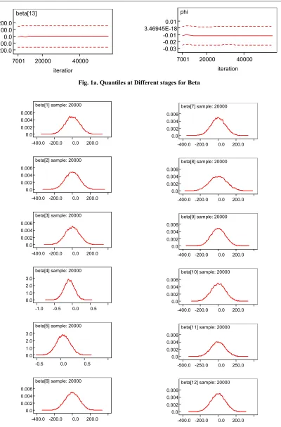
The different stages of Hierarchical Bayesian model analysis using WinBUGS is illustrated in the following tables. This is initiated at 5000 burning followed every 10000 iterations up to maximum of fifty thousand. This hierarchical model is to study the weight gain at different time period in a year and the variance of weight between regimens. The fixed effects i (i=1,2,…,13), were assumed to

[image:5.504.259.472.77.345.2]

follow vague independent normal distribution with zero mean and low precision = 0.0001. The posterior mean and standard error for each regression coefficients and the between treatment covariance are also shown in the above tables. The treatment-specific intercept measures the residual effect for a particular treatment after adjusting for patients and treatment covariates.

iterations

0.03 Median 0.98 Start Sample

T[1,1] 0.39 3.13 25.97 96.55 5001 20000 T[1,2] 0.30 -36.98 1.25 37.18 5001 20000 T[1,3] 0.31 -37.14 0.65 37.16 5001 20000 T[2,1] 0.30 -36.98 1.25 37.18 5001 20000 T[2,2] 0.37 3.22 25.50 95.18 5001 20000 T[2,3] 0.30 -37.02 0.82 35.61 5001 20000 T[3,1] 0.31 -37.14 0.65 37.16 5001 20000 T[3,2] 0.30 -37.02 0.82 35.61 5001 20000 T[3,3] 0.36 3.17 26.06 96.66 5001 20000 alpha[1,1] 1.36 -1.59 29.12 64.74 5001 20000 alpha[1,2] 1.38 -88.76 -58.10 -13.53 5001 20000 alpha[1,3] 1.96 -3.86 22.37 78.56 5001 20000 alpha[2,1] 1.36 -1.45 29.26 64.55 5001 20000 alpha[2,2] 1.38 -88.82 -58.31 -13.74 5001 20000 alpha[2,3] 1.97 -4.11 22.39 78.54 5001 20000 alpha[3,1] 1.36 -1.14 29.27 64.60 5001 20000 alpha[3,2] 1.37 -88.78 -58.29 -13.69 5001 20000 alpha[3,3] 1.97 -4.26 22.65 78.71 5001 20000 beta[1] 0.50 -158.50 -1.05 159.80 5001 20000 beta[2] 0.57 -159.00 0.51 160.30 5001 20000 beta[3] 0.53 -160.00 -0.01 159.10 5001 20000 beta[4] 0.00 -0.38 -0.09 0.20 5001 20000 beta[5] 0.00 -0.22 0.06 0.34 5001 20000 beta[6] 0.58 -158.70 0.41 157.30 5001 20000 beta[7] 0.55 -161.40 -0.23 160.80 5001 20000 beta[8] 0.66 -193.60 0.14 197.40 5001 20000 beta[9] 0.51 -156.90 0.08 159.80 5001 20000 beta[10] 0.56 -158.80 0.91 160.70 5001 20000 beta[11] 0.79 -192.70 -1.46 195.40 5001 20000 beta[12] 0.59 -159.50 -0.31 157.20 5001 20000 beta[13] 0.56 -160.00 -0.51 158.30 5001 20000 phi 0.00 -0.03 -0.01 0.00 5001 20000 theta 0.03 -0.26 1.06 2.32 5001 20000

iterations

[image:5.504.260.470.369.634.2]

(6)

beta[1]

iteration

7001 20000 40000

-200.0 -100.0 0.0 100.0 200.0

beta[2]

iteration

7001 20000 40000

-200.0 -100.0 0.0 100.0 200.0

beta[3]

iteration

7001 20000 40000

-200.0 -100.0 0.0 100.0 200.0

beta[4]

iteration

7001 20000 40000

-0.4 -0.2 0.0 0.2

beta[5]

iteration

7001 20000 40000

-0.4 -0.2 0.0 0.2 0.4

beta[6]

iteration

7001 20000 40000

-200.0 -100.0 0.0 100.0 200.0

beta[7]

iteration

7001 20000 40000

-200.0 -100.0 0.0 100.0 200.0

beta[8]

iteration

7001 20000 40000

-200.0 -100.0 0.0 100.0 200.0

beta[9]

iteration

7001 20000 40000

-200.0 -100.0 0.0 100.0 200.0

beta[10]

iteration

7001 20000 40000

-200.0 -100.0 0.0 100.0 200.0

beta[11]

iteration

7001 20000 40000

-200.0 0.0 200.0 400.0

beta[12]

iteration

7001 20000 40000

(7)

phi

iteration

7001 20000 40000

-0.03 -0.02 -0.01 3.46945E-18 0.01 beta[13]

iteration

7001 20000 40000

[image:7.504.49.449.48.655.2] [image:7.504.43.470.50.153.2] [image:7.504.284.417.187.649.2]

-200.0 -100.0 0.0 100.0 200.0

Fig. 1a. Quantiles at Different stages for Beta

beta[1] sample: 20000

-400.0 -200.0 0.0 200.0 0.0

0.002 0.004 0.006

-400.0 -200.0 0.0 200.0 0.0

0.002 0.004 0.006

-400.0 -200.0 0.0 200.0 0.0

0.002 0.004 0.006

-1.0 -0.5 0.0 0.5 0.0

1.0 2.0 3.0

-0.5 0.0 0.5 0.0

1.0 2.0 3.0

-400.0 -200.0 0.0 200.0 0.0

0.002 0.004 0.006

-400.0 -200.0 0.0 200.0 0.0

0.002 0.004 0.006

-400.0 -200.0 0.0 200.0 0.0

0.002 0.004 0.006

-400.0 -200.0 0.0 200.0 0.0

0.002 0.004 0.006

-400.0 -200.0 0.0 200.0 0.0

0.002 0.004 0.006

-500.0 -250.0 0.0 250.0 0.0

0.002 0.004 0.006

-400.0 -200.0 0.0 200.0 0.0

(8)

DISCUSSION

The different stages of Hierarchical Bayesian model analysis using WinBUGS the posterior mean and standard error for each regression coefficients and the between treatment covariance are also shown in the above tables. This is initiated at 5000 burning followed every 10000 iterations up to maximum of fifty thousand. The optimum we reached at the stage of 30,000th iteration. This hierarchical model is to study the weight gain at different time period in a year and the variance of weight between regimens. The fixed effects i

(i=1,2,…,13), were assumed to follow vague independent normal distribution with zero mean and low precision = 0.0001. The posterior mean and standard error for each regression coefficients and the between treatment covariance are also shown in the above tables. The treatment- specific intercept measures the residual effect for a

particular treatment after adjusting for patients and treatment covariates. For each observation in the validation set, the predictive density is estimated by the model density averaged across parameter values in the posterior sample. The treatment-specific intercept measures the residual effect for a particular treatment after adjusting for patients and treatment covariates. The interval estimates illustrate the large degree of uncertainty associated with `league tables'; There is no much diffrence between the tratments . We also note that the treatment mean is also closely identical to the mean of intercepts.

REFERENCES

Berliner, L.M. 1996. Hierarchical Bayesian time series models. Proceeding of the XVth

-400.0 -200.0 0.0 200.0 0.0

0.002 0.004 0.006

phi sample: 20000

-0.06 -0.02 0.02 0.0

[image:8.504.72.419.54.126.2]

20.0 40.0 60.0

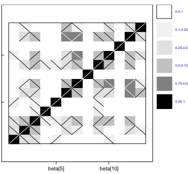
Fig. 1b. Kernal Densities at Different stages for Beta

beta[5] beta[10]

0-0.1

0.1-0.25

0.25-0.5

0.5-0.75

0.75-0.9

0.95-1

[image:8.504.161.349.164.338.2]

(9)

workshop on Maximum Entropy and Bayesian

Methods.

Carlin, B. P., and Polson, N. G. 1991. Inference for non-conjugate Bayesian models using the Gibbs Sampler, Canadian Journal of Statistics, 19: 399-405.

Carlin, B. P., Gelfand, A. E., and Smith, A. F. M. 1992. Hierarchical Bayesian analysis of change point problems, Journal of the Royal Statistical

Society, C, 41, 389-405.

Casella, G., and George, E.I. 1992. Explaining the Gibbs sampler. The American Statistician,

46:167-74.

Chib, S., and Greenberg, E. 1995. Understatnding the Metropolis-Hastings algorithm. The

American Statistician, 49: 327-335.

Cressie, N., and Mugglin, A. S. 2000. Spatio temporal hierarchical modeling of an infectious disease from (simulated) count data, COMPSTAT, proceedings in Computational

Statistics, Physica-Verlag, Hiedberg.

Gelfand, A. E., Smith, A. F. M., and Lee, T. M. 1992. Bayesian analysis of constrained parameter and truncated data problems, Journal

of the American Statistical Association, 87:

523-32.

Gelfand, A.E., and Smith, A.F.M. 1990. Sampling-based approaches to calculating marginal densities. Journal of the Americal

Statistical Association, 85: 398-409.

Gelfand, A.E., and Smith, A.F.M. 1991. Gibbs sampling for marginal posterior expectations,

Communications in Statistics, A, 20, 1747-66.

Gelman, A., and Rubin, D. B. 1996. Markov Chain Monte Carlo Methods in Biostatistics,

Statistical Methods in Medical Research, 5:

339-55.

Gelman, A., Carlin, J. B., Stern, H. S., and Rubin, D. B. 1995. Bayesian data analysis. Chapman & Hall, London.

Geman, S and Geman, D. 1984. Stochastic relaxation, Gibbs distributions, and the Bayesian restoration of images. IEEE Transactions on pattern analysis and Matching

Intelligence, 6: 721-41.

Gilks, W. R. and Willd, P. 1992. Adaptive rejection sampling for Gibbs sampling, Applied

Statistics, 41: 337-48.

Gilks, W. R., Richardson, S., and Spiegelhalter, D. J. 1996. Markov Chain Monte Carlo in Practice, Chapman & Hall, London

Grenander, U. 1983. Tutorial in pattern theorey.

Technical Report. Providence, R.I: Division of

Applied Mathematics, Brown University. Hastings, W.K. 1970. Monte Carlo methods using

Markov Chains and their applications.

Biometrika, 57: 97-109.

Ibrahim, G. J., Chen, M-H., and Sinha, D. 2004. Bayesian methods for joint modeling of longitudinal and survival data with applications to cancer vaccine trials. Statistica Sinica, 14: 863-83.

Metropolis, N., Rosenbluth, A., Rosenbluth, M., Teller, A., and Teller, E. 1953. Equation of state calculations by fast computing machines.

Journal of Chemical Physics, 21: 1087-91.

Mugglin, A. S., Cressie, N., and Gemmel, I. 2000. Hierarchical statistical modeling of influenza epidemic dynamics in space and time, Department of Statistics Preprint, 662, Ohio University, Columbus, OH.

Robert, C. P. 1994. The Bayesian choice, 2nd edition, Springer-Verlag, New York.

Schervish, M.J. and Carlin, B. P. 1992. On the convergence of successive substitution sampling. Journal of Computational and

Graphical Statistics, 1, 111-27.

Tanner, M. A., and Wang, W . H 1987. The calculations of the posterior distributions by data augmentation, Journal of the American

Statistical Association, 82: 528-40.

Tierney, L. 1994. Markov Chain for exploring posterior distributions, (with discussion), The

Annals of Statistics, 22: 1701-762.