A Compositional and Interpretable Semantic Space
Alona Fyshe,1 Leila Wehbe,1 Partha Talukdar,2Brian Murphy,3 and Tom Mitchell1 1 Machine Learning Department, Carnegie Mellon University, Pittsburgh, USA
2Indian Institute of Science, Bangalore, India 3 Queen’s University Belfast, Belfast, Northern Ireland
[email protected], [email protected], [email protected], [email protected], [email protected]
Abstract
Vector Space Models (VSMs) of Semantics are useful tools for exploring the semantics of single words, and the composition of words to make phrasal meaning. While many meth-ods can estimate the meaning (i.e. vector) of a phrase, few do so in an interpretable way. We introduce a new method (CNNSE) that al-lows word and phrase vectors to adapt to the notion of composition. Our method learns a VSM that is both tailored to support a chosen semantic composition operation, and whose resulting features have an intuitive interpreta-tion. Interpretability allows for the exploration of phrasal semantics, which we leverage to an-alyze performance on a behavioral task.
1 Introduction
Vector Space Models (VSMs) are models of word semantics typically built with word usage statistics derived from corpora. VSMs have been shown to closely match human judgements of semantics (for an overview see Sahlgren (2006), Chapter 5), and can be used to study semantic composition (Mitchell and Lapata, 2010; Baroni and Zamparelli, 2010; Socher et al., 2012; Turney, 2012).
Composition has been explored with different types of composition functions (Mitchell and La-pata, 2010; Mikolov et al., 2013; Dinu et al., 2013) including higher order functions (such as ma-trices) (Baroni and Zamparelli, 2010), and some have considered which corpus-derived information is most useful for semantic composition (Turney, 2012; Fyshe et al., 2013). Still, many VSMs act
like a black box - it is unclear what VSM dimen-sions represent (save for broad classes of corpus statistic types) and what the application of a com-position function to those dimensions entails. Neu-ral network (NN) models are becoming increas-ingly popular (Socher et al., 2012; Hashimoto et al., 2014; Mikolov et al., 2013; Pennington et al., 2014), and some model introspection has been attempted: Levy and Goldberg (2014) examined connections between layers, Mikolov et al. (2013) and Penning-ton et al. (2014) explored how shifts in VSM space encodes semantic relationships. Still, interpreting NN VSM dimensions, or factors, remains elusive.
This paper introduces a new method, Composi-tional Non-negative Sparse Embedding (CNNSE). In contrast to many other VSMs, our method learns aninterpretableVSM that is tailored to suit the se-mantic composition function. Such interpretability allows for deeper exploration of semantic composi-tion than previously possible. We will begin with an overview of the CNNSE algorithm, and follow with empirical results which show that CNNSE produces:
1. more interpretable dimensions than the typical VSM,
2. composed representations that outperform pre-vious methods on a phrase similarity task.
Compared to methods that do not consider composi-tion when learning embeddings, CNNSE produces:
1. better approximations of phrasal semantics, 2. phrasal representations with dimensions that
more closely match phrase meaning.
2 Method
Typically, word usage statistics used to create a VSM form a sparse matrix with many columns, too unwieldy to be practical. Thus, most models use some form of dimensionality reduction to compress the full matrix. For example, Latent Semantic Anal-ysis (LSA) (Deerwester et al., 1990) uses Singular Value Decomposition (SVD) to create a compact VSM. SVD often produces matrices where, for the vast majority of the dimensions, it is difficult to in-terpret what a high or low score entails for the se-mantics of a given word. In addition, the SVD fac-torization does not take into account the phrasal re-lationships between the input words.
2.1 Non-negative Sparse Embeddings
Our method is inspired by Non-negative Sparse Em-beddings (NNSEs) (Murphy et al., 2012). NNSE promotes interpretability by including sparsity and non-negativity constraints into a matrix factoriza-tion algorithm. The result is a VSM with extremely coherent dimensions, as quantified by a behavioral task (Murphy et al., 2012). The output of NNSE is a matrix with rows corresponding to words and columns corresponding to latent dimensions.
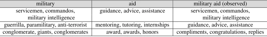
To interpret a particular latent dimension, we can examine the words with the highest numerical val-ues in that dimension (i.e. identify rows with the highest values for a particular column). Though the representations in Table 1 were created with our new method, CNNSE, we will use them to illustrate the interpretability of both NNSE and CNNSE, as the form of the learned representations is similar. One of the dimensions in Table 1 has top scoring words
guidance, adviceand assistance - words related to help and support. We will refer to these word list summaries as the dimension’s interpretable sum-marization. To interpret the meaning of a particu-lar word, we can select its highest scoring dimen-sions (i.e. choose columns with maximum values for a particular row). For example, the interpretable summarizations for the top scoring dimensions of the wordmilitaryinclude both positions in the mil-itary (e.g. commandos), and milmil-itary groups (e.g. paramilitary). More examples in Supplementary
Material (http://www.cs.cmu.edu/˜fmri/
papers/naacl2015/).
NNSE is an algorithm which seeks a lower
di-mensional representation forw words using thec -dimensional corpus statistics in a matrixX∈Rw×c. The solution is two matrices: A ∈ Rw×` that is sparse, non-negative, and represents word semantics in an `-dimensional latent space, and D ∈ R`×c: the encoding of corpus statistics in the latent space. NNSE minimizes the following objective:
argmin A,D
1 2
w
X
i=1
Xi,:−Ai,:×D2+λ
1Ai,:1
(1) st:Di,:DTi,:≤1,∀1≤i≤` (2)
Ai,j ≥0, 1≤i≤w, 1≤j≤` (3) whereAi,j indicates the entry at theith row andjth column of matrixA, andAi,:indicates theith row
of the matrix. TheL1constraint encourages sparsity
inA;λ1is a hyperparameter. Equation 2 constrains
D to eliminate solutions where the elements of A are made arbitrarily small by making the norm ofD arbitrarily large. Equation 3 ensures thatAis non-negative. Together,AandDfactor the original cor-pus statistics matrixX to minimize reconstruction error. One may tune`andλ1to vary the sparsity of
the final solution.
Murphy et al. (2012) solved this system of con-straints using the Online Dictionary Learning algo-rithm described in Mairal et al. (2010). Though Equations 1-3 represent a non-convex system, when solving forAwithDfixed (and vice versa) the loss function is convex. Mairal et al. break the prob-lem into two alternating optimization steps (solv-ing for A and D) and find the system converges to a stationary solution. The solution for A is found with a LARS implementation for lasso regres-sion (Efron et al., 2004);Dis found via gradient de-scent. Though the final solution may not be globally optimal, this method is capable of handling large amounts of data and has been shown to produce use-ful solutions in practice (Mairal et al., 2010; Murphy et al., 2012).
2.2 Compositional NNSE
Table 1: CNNSE interpretable summarizations for the top 3 dimensions of an adjective, noun and adjective-noun phrase.
military aid military aid (observed)
servicemen, commandos, guidance, advice, assistance servicemen, commandos,
military intelligence military intelligence
guerrilla, paramilitary, anti-terrorist mentoring, tutoring, internships guidance, advice, assistance conglomerate, giants, conglomerates award, awards, honors compliments, congratulations, replies
theL1 regularizer can have a large impact on
spar-sity, our composition constraint represents a consid-erable change in composition compatibility.
Consider a phrasepmade up of wordsiandj. In the most general setting, the following composition constraint could be applied to the rows of matrix A corresponding top, iandj:
A(p,:)=f(A(i,:), A(j,:)) (4) where f is some composition function. The com-position function constrains the space of learned la-tent representationsA∈Rw×`to be those solutions that are compatible with the composition function defined by f. Incorporating f into Equation 1 we have:
argmin A,D,Ω
w
X
i=1
1
2Xi,:−Ai,:×D2+λ1Ai,:1+
λc 2
X
phrasep, p=(i,j)
A(p,:)−f(A(i,:), A(j,:))2 (5)
Where each phrase p is comprised of words (i, j) andΩrepresents all parameters offto be optimized. We have added a squared loss term for composition, and a new regularization parameter λc to weight the importance of respecting composition. We call this new formulation Compositional Non-Negative Sparse Embeddings (CNNSE). Some examples of the interpretable representations learned by CNNSE for adjectives, nouns and phrases appear in Table 1.
There are many choices for f: addition, multi-plication, dilation, etc. (Mitchell and Lapata, 2010). Here we choosefto be weighted addition because it has has been shown to work well for adjective noun composition (Mitchell and Lapata, 2010; Dinu et al., 2013; Hashimoto et al., 2014), and because it lends itself well to optimization. Weighted addition is:
f(A(i,:), A(j,:)) =αA(i,:)+βA(j,:) (6)
This choice offrequires that we simultaneously op-timize forA, D, αandβ. However,αandβare sim-ply constant scaling factors for the vectors inA cor-responding to adjectives and nouns. For adjective-noun composition, the optimization ofα andβ can be absorbed by the optimization ofA. For models that include noun-noun composition, ifαandβ are assumed to be absorbed by the optimization of A, this is equivalent to settingα=β.
We can further simplify the loss function by con-structing a matrixB that imposes the composition by addition constraint. B is constructed so that for each phrasep = (i, j): B(p,p) = 1,B(p,i) = −α,
andB(p,j)=−β. For our models, we useα =β = 0.5, which serves to average the single word repre-sentations. The matrixB allows us to reformulate the loss function from Eq 5:
argmin A,D
1
2X−AD2F +λ1A1+
λc
2BA2F (7) whereF indicates the Frobenius norm. B acts as a selector matrix, subtracting from the latent represen-tation of the phrase the average latent represenrepresen-tation of the phrase’s constituent words.
We now have a loss function that is the sum of several convex functions ofA: squared reconstruc-tion loss forA, L1 regularization and the
composi-tion constraint. This sum of sub-funccomposi-tions is the for-mat required for the alternating direction method of multipliers (ADMM) (Boyd, 2010). ADMM substi-tutes a dummy variablezforAin the sub-functions:
argmin A,D
1
2X−AD
2
F +λ1z11+
λc 2 Bzc
2
F (8) and, in addition to constraints in Eq 2 and 3, incor-porates constraintsA = z1 andA = zc to ensure
dummy variables match A. ADMM uses an
mented Lagrangian to incorporate and relax these new constraints. We optimize forA, z1 andzc sep-arately, update the dual variables and repeat until convergence (see Supplementary material for La-grangian form, solutions and updates). We modi-fied code for ADMM, which is available online1. ADMM is used when solving for A in the Online Dictionary Learning algorithm, solving for D re-mains unchanged from the NNSE implementation (see Algorithms 1 and 2 in Supplementary Material). We use the weighted addition composition func-tion because it performed well for adjective-noun composition in previous work (Mitchell and Lap-ata, 2010; Dinu et al., 2013; Hashimoto et al., 2014), maintains the convexity of the loss function, and is easy to optimize. In contrast, an element-wise mul-tiplication, dilation or higher-order matrix compo-sition function will lead to a non-convex optimiza-tion problem which cannot be solved using ADMM. Though not explored here, we hypothesize that A could be molded to respect many different compo-sition functions. However, if the chosen composi-tion funccomposi-tion does not maintain convexity, finding a suitable solution forAmay prove challenging. We also hypothesize that even if the chosen composi-tion funccomposi-tion is not the “true” composicomposi-tion funccomposi-tion (whatever that may be), the fact thatA can change to suit the composition function may compensate for this mismatch. This has the flavor of variational in-ference for Bayesian methods: an approximation in place of an intractable problem often yields better results with limited data, in less time.
3 Data and Experiments
We use the semantic vectors made available by Fyshe et al. (2013), which were compiled from a 16 billion word subset of ClueWeb09 (Callan and Hoy, 2009). We used the 1000 dependency SVD dimen-sions, which were shown to perform well for compo-sition tasks. Dependency features are tuples consist-ing of two POS tagged words and their dependency relationship in a sentence; the feature value is the pointwise positive mutual information (PPMI) for the tuple. The dataset is comprised of 54,454 words and phrases. We randomly split the approximately 14,000 adjective noun phrases into a train (2/3) and
1http://www.stanford.edu/˜boyd/papers/
[image:4.612.323.530.147.218.2]admm/
Table 2: Median rank, mean reciprocal rank (MRR) and percentage of test phrases ranked perfectly (i.e. first in a sorted list of approx. 4,600 test phrases) for four methods of estimating the test phrase vec-tors. w.addSVDis weighted addition of SVD vectors, w.addNNSEis weighted addition of NNSE vectors.
Model Med. Rank MRR Perfect
w.addSVD 99.89 35.26 20%
w.addNNSE 99.80 28.17 16%
Lexfunc 99.65 28.96 20%
CNNSE 99.91 40.65 26%
test (1/3) set. From the test set we removed 200 ran-domly selected phrases as a development set for pa-rameter tuning. We did not lexically split the train and test sets, so many words appearing in training phrases also appear in test phrases. For this reason we cannot make specific claims about the generaliz-ability of our methods to unseen words.
NNSE has one parameter to tune (λ1); CNNSE
has two: λ1 andλc. In general, these methods are
not overly sensitive to parameter tuning, and search-ing over orders of magnitude will suffice. We found the optimal settings for NNSE wereλ1 = 0.05, and
for CNNSE λ1 = 0.05, λc = 0.5. Too large λ1
leads to overly sparse solutions, too small reduces interpretability. We set ` = 1000 for both NNSE and CNNSE and altered sparsity by tuning onlyλ1.
3.1 Phrase Vector Estimation
To test the ability of each model to estimate phrase semantics we trained models on the training set, and used the learned model and the composition function to estimate vectors of held out phrases. We sort the vectors for the test phrases, Xtest, by their cosine distance to the predicted phrase vectorXˆ(p,:).
We report two measures of accuracy. The first is median rank accuracy. Rank accuracy is:100×(1−
r
P), where r is the position of the correct phrase in the sorted list of test phrases, and P = |Xtest| (the number of test phrases). The second measure is mean reciprocal rank (MRR), which is often used to evaluate information retrieval tasks (Kantor and Voorhees, 2000). MRR is
100×(P1 XP i=1
For both rank accuracy and MRR, a perfect score is 100. However, MRR places more emphasis on rank-ing items close to the top of the list, and less on dif-ferences in ranking lower in the list. For example, if the correct phrase is always ranked 2, 50 or 100 out of list of 4600, median rank accuracy would be 99.95, 98.91or97.83. In contrast, MRR would be 50, 2 or1. Note that rank accuracy and reciprocal rank produce identical orderings of methods. That is, whatever method performs best in terms of rank accuracy will also perform best in terms of recip-rocal rank. MRR simply allows us to discriminate between very accurate models. As we will see, the rank accuracy of all models is very high (> 99%), approaching the rank accuracy ceiling.
3.1.1 Estimation Methods
We will compare to two other previously studied composition methods: weighted addition (w.addSVD), and lexfunc (Baroni and Zamparelli, 2010). Weighted addition findsα, βto optimize
(X(p,:)−(αX(i,:)+βX(j,:)))2
Note that this optimization is performed over the SVD matrix X, rather than onA. To estimateX for a new phrasep= (i, j)we compute
ˆ
X(p,:)=αX(i,:)+βX(j,:)
Lexfunc finds an adjective-specific matrix Mi that solves
X(p,:) =MiX(j,:)
for all phrasesp = (i, j)for adjectivei. We solved each adjective-specific problem with Matlab’s par-tial least squares implementation, which uses the SIMPLS algorithm (Dejong, 1993). To estimateX for a new phrasep= (i, j)we compute
ˆ
X(p,:) =MiX(j,:)
We also optimized the weighted addition compo-sition function over NNSE vectors, which we call
w.addNNSE. After optimizing α and β using the training set, we compose the latent word vectors to estimate the held out phrase:
ˆ
A(p,:) =αA(i,:)+βA(j,:)
For CNNSE, as in the loss function,α = β = 0.5 so that the average of the word vectors approximates
the phrase. ˆ
A(p,:) = 0.5×(A(i,:)+A(j,:))
Crucially, w.addNNSE estimates α, β after learning the latent spaceA, whereas CNNSEsimultaneously
learns the latent space A, while taking the compo-sition function into account. Once we have an esti-mateAˆ(p,:)we can use the NNSE and CNNSE
solu-tions forDto estimate the corpus statistics X. ˆ
X(p,:) = ˆA(p,:)D
Results for the four methods appear in Table 2. Median rank accuracies were all within half a per-centage point of each other. However, MRR shows a striking difference in performance. CNNSE has MRR of 40.64, more than 5 points higher than the second highest MRR score belonging to w.addSVD (35.26). CNNSE ranks the correct phrase in the first position for26%of phrases, compared to20% for w.addSVD. Lexfunc ranks the correct phrase first for 20% of the test phrases, w.addNNSE 16%. So, while all models perform quite well in terms of rank accuracy, when we use the more discrim-inative MRR, CNNSE is the clear winner. Note that the performance of w.addNNSE is much lower than CNNSE. Incorporating a composition con-straint into the learning algorithm has produced a la-tent space that surpasses all methods tested for this task.
We were surprised to find that lexfunc performed relatively poorly in our experiments. Dinu et al. (2013) used simple unregularized regression to es-timateM. We also replicated that formulation, and found phrase ranking to be worse when compared to the Partial Least Squares method described in Ba-roni and Zamparelli (2010). In addition, BaBa-roni and Zamparelli use 300 SVD dimensions to estimateM. We found that, for our dataset, using all 1000 dimen-sions performed slightly better.
require only that the adjective appear in the train-ing data). To compensate for this possibly unfair train/test split, the results in Table 2 are calculated over only those adjectives which could be estimated using the training set.
Though the results reported here are not as high as previously reported, lexfunc was found to be only slightly better than w.addSVDfor adjective noun composition (Dinu et al., 2013). CNNSE outper-forms w.addSVD by a large margin, so even if Lex-func could be tuned to perform at previous levels on this dataset, CNNSE would likely still dominate.
3.1.2 Phrase Estimation Errors
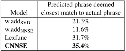
None of the models explored here are perfect. Even the top scoring model, CNNSE, only identi-fies the correct phrase for 26% of the test phrases. When a model makes a “mistake”, it is possible that the top-ranked phrase is a synonym of, or closely related to, the actual phrase. To evaluate mistakes, we chose test phrases for which all 4 models are in-correct and produce a different top ranked phrase (likely these are the most difficult phrases to es-timate). We then asked Mechanical Turk (Mturk http://mturk.com) users to evaluate the mis-takes. We presented the 4 mistakenly top-ranked phrases to Mturk users, who were asked to choose the one phrase most related to the actual test phrase. We randomly selected 200 such phrases and asked 5 Mturk users to evaluate each, paying $0.01 per an-swer. We report here the results for questions where a majority (3) of users chose the same answer (82% of questions). For all Mturk experiments described in this paper, a screen shot of the question appears in the Supplementary Material.
[image:6.612.324.530.156.240.2]Table 3 shows the Mturk evaluation of model mis-takes. CNNSE and lexfunc make the most reason-able mistakes, having their top-ranked phrase cho-sen as the most related phrase 35.4% and 31.7% of the time, respectively. This makes us slightly more comfortable with our phrase estimation results (Ta-ble 2); though lexfunc does not reliably predict the correct phrase, it often chooses a close approxima-tion. The mistakes from CNNSE are chosen slightly more often than lexfunc, indicating that CNNSE also has the ability to reliably predict the correct phrase, or a phrase deemed more related than those chosen by other methods.
Table 3: A comparison of mistakes in phrase rank-ing across 4 composition methods. To evaluate mis-takes, we chose phrases for which all 4 models rank a different (incorrect) phrase first. Mturk users were asked to identify the phrase that was semantically closest to the target phrase.
Predicted phrase deemed Model closest match to actual phrase
w.addSVD 21.3%
w.addNNSE 11.6%
Lexfunc 31.7%
CNNSE 35.4%
3.2 Interpretability
Though our improvement in MRR for phrase vec-tor estimation is compelling, we seek to explore the meaning encoded in the word space features. We turn now to theinterpretation of phrasal semantics and semantic composition.
3.2.1 Interpretability of Latent Dimensions
Due to the sparsity and non-negativity constraints, NNSE produces dimensions with very coherent se-mantic groupings (Murphy et al., 2012). Murphy et al. used an intruder task to quantify the inter-pretability of semantic dimensions. The intruder task presents a human user with a list of words, and they are to choose the one word that does not belong in the list (Chang et al., 2009). For example, from the list (red, green, desk, pink, purple, blue), it is clear to see that the word “desk” does not belong in the list of colors.
Table 4: Quantifying the interpretability of learned semantic representations via the intruder task. In-truders detected: % of questions for which the ma-jority response was the intruder. Mturk agreement: the % of questions for which a majority of users chose the same response.
Method Intruders Detected Mturk Agreement
SVD 17.6% 74%
NNSE 86.2% 94%
CNNSE 88.9% 90%
representationX, SVD interpretability is a proxy for lexfunc interpretability.
Results for the intruder task appear in Table 4. Consistent with previous studies, NNSE provides a much more interpretable latent representation than SVD. We find that the additional composition con-straint used in CNNSE has maintained the inter-pretability of the learned latent space. Because in-truders detected is higher for CNNSE, but agreement amongst Mturk users is higher for NNSE, we con-sider the interpretability results for the two methods to be equivalent. Note that SVD interpretability is close to chance (1/6 = 16.7%).
3.2.2 Coherence of Phrase Representations
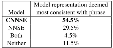
The dimensions of NNSE and CNNSE are com-parably interpretable. But, has the composition con-straint in CNNSE resulted in better phrasal repre-sentations? To test this, we randomly selected 200 phrases, and then identified the top scoring dimen-sion for each phrase in both the NNSE and CNNSE models. We presented Mturk users with the inter-pretable summarizations for these top scoring di-mensions. Users were asked to select the list of words (interpretable summarization) most closely related to the target phrase. Mturk users could also select that neither list was related, or that the lists were equally related to the target phrase. We paid $0.01 per answer and had 5 users answer each question. In Table 5 we report results for phrases where the majority of users selected the same an-swer (78% questions). CNNSE phrasal represen-tations are found to be much more consistent, re-ceiving a positive evaluation almost twice as often as NNSE.
Together, these results show that CNNSE repre-sentations maintain the interpretability of NNSE
di-Table 5: Comparing the coherence of phrase rep-resentations from CNNSE and NNSE. Mturk users were shown the interpretable summarization for the top scoring dimension of target phrases. Represen-tations from CNNSE and NNSE were shown side by side and users were asked to choose the list (summa-rization) most related to the phrase, or that the lists were equally good or bad.
Model representation deemed
Model most consistent with phrase
CNNSE 54.5%
NNSE 29.5%
Both 4.5%
Neither 11.5%
mensions, while improving the coherence of phrase representations.
3.3 Evaluation on Behavioral Data
We now compare the performance of various com-position methods on an adjective-noun phrase sim-ilarity dataset (Mitchell and Lapata, 2010). This dataset is comprised of 108 adjective-noun phrase pairs split into high, medium and low similarity groups. Similarity scores from 18 human subjects are averaged to create one similarity score per phrase pair. We then compute the cosine similarity between the composed phrasal representations of each phrase pair under each compositional model. As in Mitchell and Lapata (2010), we report the correlation of the cosine similarity measures to the behavioral scores. We withheld 12 of the 108 questions for parame-ter tuning, four randomly selected from each of the high, medium and low similarity groups.
Table 6 shows the correlation of each model’s similarity scores to behavioral similarity scores. Again, Lexfunc performs poorly. This is proba-bly attributable to the fact that there are, on aver-age, only 39 phrases available for training each ad-jective in the dataset, whereas the original Lexfunc study had at least 50 per adjective (Baroni and Zam-parelli, 2010). CNNSE is the top performer, fol-lowed closely by weighted addition. Interestingly, weighted NNSE correlation is lower than CNNSE by nearly 0.15, which shows the value of allowing the learned latent space to conform to the desired composition function.
[image:7.612.327.525.175.260.2]3.3.1 Interpretability and Phrase Similarity
CNNSE has the additional advantage of inter-pretability. To illustrate, we created a web page to explore the dataset under the CNNSE model.
The pagehttp://www.cs.cmu.edu/˜fmri/
papers/naacl2015/cnnse_mitchell_ lapata_all.html displays phrase pairs sorted
by average similarity score. For each phrase
in the pair we show a summary of the CNNSE composed phrase meaning. The scores of the 10 top dimensions are displayed in descending order. Each dimension is described by its interpretable summarization. As one scrolls down the page, the similarity scores increase, and the number of dimen-sions shared between the phrase pairs (highlighted in red) increases. Some phrase pairs with high similarity scores share no top scoring dimensions. Because we can interpret the dimensions, we can begin to understand how the CNNSE model is failing, and how it might be improved.
For example, the phrase pair judged most similar by the human subjects, but that shares none of the top 10 dimensions in common, is “large number” and “great majority” (behavioral similarity score 5.61/7). Upon exploration of CNNSE phrasal repre-sentations, we see that the representation for “great majority” suffers from the multiple word senses of majority. Majority is often used in political settings to describe the party or group with larger member-ship. We see that the top scoring dimension for “great majority” has top scoring words “candidacy, candidate, caucus”, a politically-themed dimension. Though the CNNSE representation is not incorrect for the word, the common theme between the two test phrases is not political.
[image:8.612.358.497.107.192.2]The second highest scoring dimension for “large number” is “First name, address, complete address”. Here we see another case of the collision of multiple word senses, as this dimension is related to identify-ing numbers, rather than the quantity-related sense of number. While it is satisfying that the word senses for majority and number have been separated out into different dimensions for each word, it is clear that both the composition and similarity functions used for this task are not gracefully handling multi-ple word senses. To address this issue, we could par-tition the dimensions ofAinto sense-related groups
Table 6: Correlation of phrase similarity judgements (Mitchell and Lapata, 2010) to pairwise distances in several adjective-noun composition models.
Correlation to
Model behavioral data
w.addSVD 0.5377
w.addNNSE 0.4469
Lexfunc 0.1347
CNNSE 0.5923
and use the maximally correlated groups to score phrase pairs. CNNSE interpretability allows us to perform these analyses, and will also allow us to it-erate and improve future compositional models.
4 Conclusion
We explored a new method to create an interpretable VSMs that respects the notion of semantic compo-sition. We found that our technique for incorporat-ing phrasal relationship constraints produced a VSM that is more consistent with observed phrasal repre-sentations and with behavioral data.
We found that, compared to NNSE, human eval-uators judged CNNSE phrasal representations to be a better match to phrase meaning. We leveraged this improved interpretability to explore composition in the context of a previously published compositional task. We note that the collision of word senses of-ten hinders performance on the behavioral data from Mitchell and Lapata (2010).
More generally, we have shown that incorporat-ing constraints to represent the task of interest can improve a model’s performance on that task. Ad-ditionally, incorporating such constraints into an in-terpretablemodel allows for a deeper exploration of performance in the context of evaluation tasks.
Acknowledgments
This work was supported in part by a gift from Google, NIH award 5R01HD075328, IARPA award FA865013C7360, DARPA award FA8750-13-2-0005, and by a fellowship to Alona Fyshe from the Multimodal Neuroimaging Training Program (NIH awards T90DA022761 and R90DA023420).
References
adjective-noun constructions in semantic space. In Proceedings of the 2010 Conference on Em-pirical Methods in Natural Language Processing, pages 1183–1193. Association for Computational Linguistics, 2010.
Stephen Boyd. Distributed Optimization and Sta-tistical Learning via the Alternating Direction Method of Multipliers. Foundations and Trends in Machine Learning, 3(1):1–122, 2010. ISSN 1935-8237. doi: 10.1561/2200000016.
Jamie Callan and Mark Hoy. The ClueWeb09
Dataset, 2009. URL http://boston.lti.
cs.cmu.edu/Data/clueweb09/.
Jonathan Chang, Jordan Boyd-Graber, Sean Gerrish, Chong Wang, and David M Blei. Reading Tea Leaves : How Humans Interpret Topic Models. In
Advances in Neural Information Processing Sys-tems, pages 1–9, 2009.
Scott Deerwester, Susan T. Dumais, George W. Fur-nas, Thomas K. Landauer, and Richard Harsh-man. Indexing by Latent Semantic Analysis.
Journal of the American Society for Information Science, 41(6):391–407, 1990.
S Dejong. SIMPLS - An alternative approach to partial least squares regression. Chemometrics and Intelligent Laboratory Systems, 18(3):251– 263, 1993. ISSN 01697439. doi: 10.1016/ 0169-7439(93)85002-x.
Georgiana Dinu, Nghia The Pham, and Marco Ba-roni. General estimation and evaluation of com-positional distributional semantic models. In
Workshop on Continuous Vector Space Models and their Compositionality, Sofia, Bulgaria, 2013. Bradley Efron, Trevor Hastie, Iain Johnstone, and Robert Tibshirani. Least angle regression. Annals of Statistics, 32(2):407–499, 2004.
Alona Fyshe, Partha Talukdar, Brian Murphy, and Tom Mitchell. Documents and Dependencies : an Exploration of Vector Space Models for Seman-tic Composition. InComputational Natural Lan-guage Learning, Sofia, Bulgaria, 2013.
Kazuma Hashimoto, Pontus Stenetorp, Makoto Miwa, and Yoshimasa Tsuruoka. Jointly learn-ing word representations and composition func-tions using predicate-argument structures. Pro-ceedings of the Conference on Empirical Methods
on Natural Language Processing, pages 1544– 1555, 2014.
Paul B. Kantor and Ellen M. Voorhees. The TREC-5 Confusion Track: Comparing Retrieval Methods for Scanned Text. Information Retrieval, 2:165– 176, 2000. ISSN 1386-4564, 1573-7659. doi: 10.1023/A:1009902609570.
Omer Levy and Yoav Goldberg. Neural Word Em-bedding as Implicit Matrix Factorization. In Ad-vances in Neural Information Processing Sys-tems, pages 1–9, 2014.
Julien Mairal, Francis Bach, J Ponce, and Guillermo Sapiro. Online learning for matrix factoriza-tion and sparse coding. The Journal of Machine Learning Research, 11:19–60, 2010.
Tomas Mikolov, Ilya Sutskever, Kai Chen, Greg Corrado, and Jeff Dean. Distributed representa-tions of words and phrases and their composition-ality. InProceedings of Neural Information Pro-cessing Systems, pages 1–9, 2013.
Jeff Mitchell and Mirella Lapata. Composition in distributional models of semantics. Cogni-tive science, 34(8):1388–429, November 2010.
ISSN 1551-6709. doi: 10.1111/j.1551-6709.
2010.01106.x.
Brian Murphy, Partha Talukdar, and Tom Mitchell. Learning Effective and Interpretable Semantic Models using Non-Negative Sparse Embedding. InProceedings of Conference on Computational Linguistics (COLING), 2012.
Jeffrey Pennington, Richard Socher, and Christo-pher D Manning. GloVe : Global Vectors for Word Representation. In Conference on Empir-ical Methods in Natural Language Processing, Doha, Qatar, 2014.
Magnus Sahlgren. The Word-Space Model Using
distributional analysis to represent syntagmatic and paradigmatic relations between words. Doc-tor of philosophy, Stockholm University, 2006. Richard Socher, Brody Huval, Christopher D.
Man-ning, and Andrew Y. Ng. Semantic Composition-ality through Recursive Matrix-Vector Spaces. InConference on Empirical Methods in Natural Language Processing and Computational Natural Language Learning, 2012.
Peter D Turney. Domain and Function : A Dual-Space Model of Semantic Relations and Com-positions. Journal of Artificial Intelligence Re-search, 44:533–585, 2012.