UniMelb NLP CORE: Integrating predictions from multiple domains and feature sets for estimating semantic textual similarity

UniMelb NLP-CORE: Integrating predictions from multiple domains and

feature sets for estimating semantic textual similarity

Spandana Gella,♣Bahar Salehi,♠♣Marco Lui,♠♣ Karl Grieser,♣Paul Cook,♣ and Timothy Baldwin,♠♣

♠NICTA Victoria Research Laboratory

♣Department of Computing and Information Systems, The University of Melbourne

[email protected], [email protected] [email protected], [email protected]

[email protected], [email protected]

Abstract

In this paper we present our systems for cal-culating the degree of semantic similarity be-tween two texts that we submitted to the Se-mantic Textual Similarity task at SemEval-2013. Our systems predict similarity using a regression over features based on the fol-lowing sources of information: string similar-ity, topic distributions of the texts based on latent Dirichlet allocation, and similarity be-tween the documents returned by an informa-tion retrieval engine when the target texts are used as queries. We also explore methods for integrating predictions using different training datasets and feature sets. Our best system was ranked 17th out of 89 participating systems. In our post-task analysis, we identify simple changes to our system that further improve our results.

1 Introduction

Semantic Textual Similarity (STS) measures the de-gree of semantic similarity or equivalence between a pair of short texts. STS is related to many natural language processing applications such as text sum-marisation (Aliguliyev, 2009), machine translation, word sense disambiguation, and question answering (De Boni and Manandhar, 2003; Jeon et al., 2005).

Two short texts are considered similar if they both convey similar messages. Often it is the case that similar texts will have a high degree of lexical over-lap, although this isn’t always so. For example,

SC dismissed government’s review plea in Vodafone tax caseandSC dismisses govt’s review petition on Vodafone tax verdictare semantically similar. These

texts have matches in terms of exact words (SC,

Vodafone,tax), morphologically-related words ( dis-missed and dismisses), and abbreviations ( govern-ment’sandgovt’s). However, the usages (senses) of

pleaandpetition, andcaseandverdictare also sim-ilar.

One straightforward way of estimating semantic similarity of two texts is by using approaches based on the similarity of the surface forms of the words they contain. However, such methods are not capa-ble of capturing similarity or relatedness at the lexi-cal level, and moreover, they do not exploit the con-text in which individual words are used in a target text. Nevertheless, a variety of knowledge sources — including part-of-speech, collocations, syntax, and domain — can be used to identify the usage or sense of words in context (McRoy, 1992; Agirre and Martinez, 2001; Agirre and Stevenson, 2006) to ad-dress these issues.

Despite their limitations, string similarity mea-sures have been widely used in previous seman-tic similarity tasks (Agirre et al., 2012; Islam and Inkpen, 2008). Latent variable models have also been used to estimate the semantic similarity be-tween words, word usages, and texts (Steyvers and Griffiths, 2007; Lui et al., 2012; Guo and Diab, 2012; Dinu and Lapata, 2010).

In this paper, we consider three different ways of measuring semantic similarity based on word and word usage similarity:

1. String-based similarity to measure surface-level lexical similarity, taking into account morphology and abbreviations (e.g.,dismisses

anddismissed, andgovernment’sandgovt’s);

2. Latent variable models of similarity to cap-ture words that have different surface forms, but that have similar meanings or that can be used in similar contexts (e.g.,petitionandplea,

verdictandcase); and

3. Topical/domain similarityof the texts with re-spect to the similarity of documents in an ex-ternal corpus (based on information-retrieval methods) that are relevant to the target texts.

We develop features based on all three of these knowledge sources to capture semantic similarity from a variety of perspectives. We build a regres-sion model, trained on STS training data which has semantic similarity scores for pairs of texts, to learn weights for the features and rate the similarity of test instances. Our approach to the task is to explore the utility of novel features or features that have not per-formed well in previous research, rather than com-bine these features with the myriad of features that have been proposed by others for the task.

2 Text Similarity Measures

In this section we describe the various features used in our system.

2.1 String Similarity Measures (SS)

Our first set of features contains various string simi-larity measures (SS), which compare the target texts in terms of the words they contain and the order of the words (Islam and Inkpen, 2008). In the Se-mEval 2012 STS task (Agirre et al., 2012) such features were used by several participants (Biggins et al., 2012; B¨ar et al., 2012; Heilman and Mad-nani, 2012), including the first-ranked team (B¨ar et al., 2012) who considered string similarity measures alongside a wide range of other features.

For our string similarity features, the texts were lemmatized using the implementation of Lancaster Stemming in NLTK 2.0 (Bird, 2006), and all punc-tuation was removed. Limited stopword removal was carried out by eliminating the wordsa,and, and

the. The output of each string similarity measure is normalized to the range of [0,1], where 0 indi-cates that the texts are completely different, while 1 means they are identical. The normalization method for each feature is described in Salehi and Cook (to

appear), wherein the authors applied string similar-ity measures successfully to the task of predicting the compositionality of multiword expressions.

Identical Unigrams (IU): This feature measures the number of words shared between the two texts, irrespective of word order.

Longest Common Substring (LCS): This mea-sures the longest sequence of words shared between the two texts. For example, the longest common substring between the following sentences is bolded:

A woman and man are dancing in the

rain.

A coupleare dancing in thestreet.

Levenshtein (LEV1): Levenshtein distance (also known as edit distance) calculates the number of basic word-level edit operations (insertion, deletion and substitution) to transform one text into the other:

Levenshtein with substitution penalty (LEV2):

This feature is a variant of LEV1 in which substi-tution is considered as two edit operations: an inser-tion and a deleinser-tion (Baldwin, 2009).

Smith Waterman (SW): This method is designed to locally align two sequences of amino acids (Smith and Waterman, 1981). The algorithm looks for the longest similar regions by maximizing the num-ber of matches and minimizing the numnum-ber of in-sertion/deletion/substitution operations necessary to align the two sequences. In other words, it finds the longest common sequence while tolerating a small number of differences. We call this sequence, the “aligned sequence”. It has length equal to or greater than the longest common sequence.

Not Aligned Words (NAW): As mentioned above, SW looks for similar regions in the given texts. Our last string similarity feature shows the number of identical words not aligned by the SW al-gorithm. We used this feature to examine how simi-lar the unaligned words are.

2.2 Topic Modelling Similarity Measures (TM)

The topic modelling features (TM) are based on La-tent Dirichlet Allocation (LDA), a generative prob-abilistic model in which each document is mod-eled as a distribution over a finite set of topics, and each topic is represented as a distribution over words (Blei et al., 2003). We build a topic model on a back-ground corpus, and then for each target text we cre-ate a topic vector based on the topic allocations of its content words, based on the method developed by Lui et al. (2012) for predicting word usage simi-larity.

The choice of the number of topics, T, can have a big impact on the performance of this method. Choosing a small T might give overly-broad topics, while a large T might lead to un-interpretable topics (Steyvers and Griffiths, 2007). Moreover smaller numbers of topics have been shown to perform poorly on both sentence simi-larity (Guo and Diab, 2012) and word usage sim-ilarity tasks (Lui et al., 2012). We therefore build topic models for 33 values of T in the range

2,3,5,8,10,50,80,100,150,200, ...1350.

The background corpus used for generating the topic models is similar to the COL-WTMF sys-tem (Guo and Diab, 2012) from the STS-2012 task, which outperformed LDA. In particular, we use sense definitions from WordNet, Wiktionary and all sentences from the Brown corpus. Similarity be-tween two texts is measured on the basis of the simi-larity between their topic distributions. We consider three vector-based similarity measures here: Cosine similarity, Jensen-Shannon divergence and KL di-vergence. Thus for each target text pair we extract 99 features corresponding to the 3 similarity mea-sures for each of the 33T settings. These features are used as the TM feature set in the systems de-scribed below.

2.3 IR Similarity Measures (IR)

The information retrieval–based features (IR) were based on a dump of English Wikipedia from Novem-ber 2009. The entire dump was stripped of markup and tokenised using the OpenNLP tokeniser. The tokenised documents were then parsed into TREC format, with each article forming an individual doc-ument. These documents were indexed using the

Indri IR engine1 with stopword removal. Each of the two target texts was issued as a full text query (without any phrases) to Indri, and the first 1000 documents for each text were returned, based on Okapi term weighting (Robertson and Walker, 1994). These resultant document lists were then converted into features using a number of set- and rank-based measures: Dice’s coefficient, Jaccard in-dex, average overlap, and rank-biased overlap (the latter two are described in Webber et al. (2010)). The first two are based on simple set overlap and ignore the ranks; average overlap takes into account the rank, but equally weights high- and low-ranking documents; and rank-biased overlap weights higher-ranked items higher.

In addition to comparisons of the document rank-ings for a given target text pair, we also consid-ered a method that compared the top-ranking doc-uments themselves. To compare two texts, we ob-tain the top-100 documents using each text as a query as above. We then calculate the similarity be-tween these two sets of resultant documents using theχ2-based corpus similarity measure of Kilgarriff (2001). In this method theχ2 statistic is calculated for the 500 most frequent words in the union of the two sets of documents (corpora), and is interpreted as the similarity between the sets of documents.

These 5 IR features (4 rank-based, and 1 document-based) are novel in the context of STS, and are used in the compound systems described be-low.

3 Compound systems

3.1 Ridge regression

Each of our features represents a (potentially noisy) measurement of the semantic textual similarity be-tween two texts. However, the scale of our fea-tures varies, e.g.,[0,1]for the string similarity fea-tures vs. unbounded for KL divergence (one of the topic modelling features). To learn the mapping be-tween these features and the graded [0,5] scale of the shared task, we made use of a statistical tech-nique known asridge regression, as implemented in

scikit-learn.2 Ridge regression is a form of linear regression where the loss function is the

ordi-1

http://www.lemurproject.org/indri/

2

nary least squares, but with an additional L2 regular-ization term. In our empirical evaluation, we found that ridge regression outperformed linear regression on our feature set. For brevity, we only present re-sults from ridge regression.

3.2 Domain Adaptation

Domain adaptation (Daum´e and Marcu, 2006) is the general term applied to techniques for using labelled data from a related distribution to label data from a target distribution. For the 2013 Shared Task, no training data was provided for the target datasets, making domain adaptation an important considera-tion. In this work, we assume that each dataset rep-resents a different domain, and on this basis develop approaches that are sensitive to inter-domain differ-ences.

We tested two simple approaches to including do-main information in our trained model. The first ap-proach, which we will refer to asflagging, simply in-volves appending a boolean vector to each training instance to indicate which training dataset it came from. The vector has lengthD, equal to the number of training datasets (3 for this task, because we train on the STS 2012 training data). All the values of the vector are 0, except for a single 1 according to the dataset that the training instance is drawn from. For test data, the entire vector consists of 0s.

The second approach we considered is based on metalearning, and we will refer to it as domain stacking. In domain stacking, we train a regressor for each domain (the level 0 regressors (Wolpert, 1992)). Each of these regressors is then applied to a test instance to produce a predicted value (the level 0 prediction). These predictions are then com-bined using a second regressor (the level 1 regres-sor), to produce a final prediction for each instance (the level 1 prediction). This approach is closely related to feature stacking(Lui, 2012) and stacked generalization (Wolpert, 1992). A general princi-ple of metalearning is to combine multiprinci-ple weaker (“less accurate”) predictors — termed level 0 pre-dictors — to produce a stronger (“more accurate”) predictor — the level 1 predictor. In stacked gener-alization, the level 0 predictors are different learning algorithms. In feature stacking, they are the same algorithm trained on different subsets of features, in this work corresponding to different methods for

es-timating STS (Section 2). In domain stacking, the level 0 predictions are obtained from subsets of the training data, where each subset corresponds to all the instances from a single dataset (e.g. MSRpar or SMTeuroparl). In terms of subsampling the training data, this technique is related tobagging(Breiman, 1996). However, rather than generating new train-ing sets by uniform sampltrain-ing across the whole pool of training data, we treat each domain in the train-ing dataset as a unique sample. Finally, we also ex-periment withfeature-domain stacking, in which the level 0 predictions are obtained from the cross prod-uct of subsets of the training data (as per domain stacking) and subsets of the feature set (as per fea-ture stacking). We report results for all 3 variants in Section 5.

This framework of feature-domain stacking can be applied with any regression or classification al-gorithm (indeed, the level 0 and level 1 predictors could be trained using different algorithms). In this work, all our regressors are trained using ridge re-gression (Section 3.1).

4 Submitted Runs

In this section we describe the three official runs we submitted to the shared task.

4.1 Run1 — Bahar

For this run we used just the SS feature set, aug-mented with flagging for domain adaptation. Ridge regression was used to train a regressor across the three training datasets (MSRvid, MSRpar, SMTeu-roparl). Each instance was then labelled using the output of the regressor, and the output range was lin-early re-scaled to[0,5]as it occasionally produced values outside of this range. Although this approach approximates STS using only lexical textual similar-ity, it was our best-performing system on the training data (Table 1). Furthermore the SS features are ap-pealing because of their simplicity and because they do not make use of any external resources.

4.2 Run2 — Concat

FSet FL FS DS MSRpar MSRvid SMTeuroparl Ave

SS 0.522 0.537 0.526 0.528

(*) SS X 0.552 0.533 0.562 0.549

TM 0.270 0.479 0.425 0.391

TM X 0.250 0.580 0.427 0.419

IR 0.264 0.759 0.407 0.477

IR X 0.291 0.754 0.400 0.482

(+) ALL 0.401 0.543 0.513 0.485

ALL X 0.377 0.595 0.516 0.496

ALL X 0.385 0.587 0.520 0.497

ALL X 0.452 0.637 0.472 0.521

ALL X X 0.429 0.619 0.526 0.524

ALL X X 0.429 0.627 0.526 0.527

(−) ALL X X X 0.441 0.645 0.527 0.538

Table 1: Pearson’s ρ for each feature set (FSet), as well as combinations of feature sets and adap-tation strategies, on each training dataset, and the micro-average over all training datasets. (*), (+), and (−) denote Run1, Run2, and Run3, respectively, our submissions to the shared task; FL=Flagging, FS=Feature stacking, DS=Domain stacking.

was also linearly re-scaled to the [0,5]range. Un-like the previous run, the flagging approach to do-main adaptation was not used. This approach re-flects a simple application of machine learning to in-tegrating data from multiple feature sets and training datasets, and provides a useful point of comparison against more sophisticated approaches (i.e., Run3).

4.3 Run3 — Stacking

In this run, we focused on an alternative method to integrating information from multiple feature sets and training datasets, namely feature-domain stack-ing, as discussed in Section 3.2. In this approach, we train nine regressors using ridge regression on each combination of the three training datasets and three feature sets. Thus, the level 1 representation for each instance is a vector of nine predictions. For the train-ing data, when computtrain-ing the level 1 features for the same training dataset from which a given instance is drawn, 10-fold cross-validation is used. Ridge re-gression is again used to combine the level 1 repre-sentations and produce the final prediction for each instance. In addition to this, we also simultaneously apply the flagging approach to domain adaptation. This approach incorporates all of our domain adap-tation efforts, and in initial experiments on the train-ing data (Table 1) it was our second-best system.

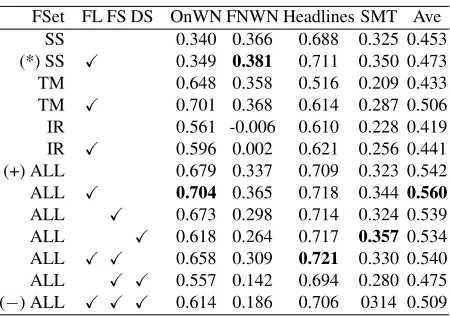
FSet FL FS DS OnWN FNWN Headlines SMT Ave SS 0.340 0.366 0.688 0.325 0.453 (*) SS X 0.349 0.381 0.711 0.350 0.473 TM 0.648 0.358 0.516 0.209 0.433 TM X 0.701 0.368 0.614 0.287 0.506 IR 0.561 -0.006 0.610 0.228 0.419 IR X 0.596 0.002 0.621 0.256 0.441 (+) ALL 0.679 0.337 0.709 0.323 0.542 ALL X 0.704 0.365 0.718 0.344 0.560 ALL X 0.673 0.298 0.714 0.324 0.539 ALL X 0.618 0.264 0.717 0.357 0.534 ALL X X 0.658 0.309 0.721 0.330 0.540 ALL X X 0.557 0.142 0.694 0.280 0.475 (−) ALL X X X 0.614 0.186 0.706 0314 0.509

Table 2: Pearson’s ρ for each feature set (FSet), as well as combinations of feature sets and adap-tation strategies, on each test dataset, and the micro-average over all test datasets. (*), (+), and (−) denote Run1, Run2, and Run3, respectively, our submissions to the shared task; FL=Flagging, FS=Feature stacking, DS=Domain stacking.

5 Results

For the STS 2013 task, the organisers advised par-ticipants to make use of the STS 2012 data; we took this to mean only thetrainingdata. In our post-task analysis, we realised that the entire 2012 dataset, in-cluding the testing data, could be used. All our of-ficial runs were trained only on the training data for the 2012 task (made up of MSRpar, MSRvid and SMTeuroparl). We first discuss preliminary find-ings training and testing on the (STS 2012) training data, and then present results for the (2013) test data. Post-submission, we re-trained our systems includ-ing the 2012 test data.

5.1 Experiments on Training Data

We evaluated our models based on a leave-one-out cross-validation across the 3 training datasets. Thus, for each of the training datasets, we trained a sep-arate model using features from the other two. We considered approaches based on each individual fea-ture set, with and without flagging. We further con-sidered combinations of feature sets using feature concatenation, as well as feature and domain stack-ing, again with and without flagging.3 Results are

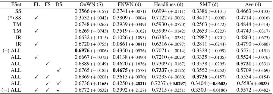
FSet FL FS DS OnWN (δ) FNWN (δ) Headlines (δ) SMT (δ) Ave (δ) SS 0.3566(+.0157) 0.3741(+.0071) 0.6994(+.0111) 0.3386(+.0131) 0.4663(+.0133) (*) SS X 0.3532(+.0042) 0.3809(−.0004) 0.7122(+.0003) 0.3417(−.0090) 0.4714(−.0016) TM 0.6748(+.0265) 0.3939(+.0349) 0.5930(+.0770) 0.2563(+.0472) 0.4844(+.0514) TM X 0.6269(−.0743) 0.3519(−.0162) 0.5999(−.0142) 0.2653(−.0223) 0.4743(−.0317) IR 0.6632(+.1015) 0.1026(+.1093) 0.6383(−.0281) 0.2987(+.0701) 0.4863(+.0673) IR X 0.6720(+.0755) 0.0861(+.0841) 0.6316(+.0097) 0.2811(+.0244) 0.4790(+.0680) (+) ALL 0.6976(+.0006) 0.4350(+.0976) 0.7071(−.0014) 0.3329(+.0099) 0.5571(+.0151) ALL X 0.6667(−.0373) 0.4138(+.0490) 0.7210(+.0029) 0.3335(−.0105) 0.5524(−.0076) ALL X 0.6889(+.0149) 0.4620(+.1636) 0.7309(+.0167) 0.3538(+.0295) 0.5721(+.0331) ALL X 0.6765(−.0185) 0.4675(+.1578) 0.7337(+.0126) 0.3552(+.0252) 0.5709(+.0369) ALL X X 0.6369(+.0208) 0.3615(+.0970) 0.7233(+.0060) 0.3736(+.0157) 0.5554(+.0154) ALL X X 0.6736(+.1165) 0.4250(+.2821) 0.7237(+0.0297) 0.3404(+0.0603) 0.5583(+.0833)

(−) ALL X X X 0.6772(+.0632) 0.3992(+.2127) 0.7315(+.0251) 0.3300(+0.0186) 0.5572(+.0482)

Table 3: Pearson’s ρ for each feature set (FSet), as well as combinations of feature sets and adaptation strategies, on eachtestdataset, and the micro-average over all test datasets, using features from all 2012 data (test + train). (*), (+), and (−) denote Run1, Run2, and Run3, respectively, our submissions to the shared task; FL=Flagging, FS=Feature stacking, DS=Domain stacking. δdenotes the difference in system performance after adding the additional training data.

reported in Table 1.

The best results on the training data were achieved using only our SS feature set with flagging (Run1), with an average Pearson’s ρ of 0.549. This fea-ture set also gave the best performance on MSR-par and SMTeuroMSR-parl, although the IR feature set was substantially better on MSRvid. On the training datasets, our approaches that combine feature sets did not give an improvement over the best individ-ual feature set on any dataset, or overall.

5.2 Test Set Results

STS 2013 included four different test sets. Table 2 presents the Pearson’s ρ for the same methods as Section 5.1 — including our submitted runs — on the test data. Run1 drops in performance on the test set as compared to the training set, where the other two runs are more consistent, suggesting that lexi-cal similarity does not generalise well cross-domain. Table 4 shows that all of our systems performed above the baseline on each dataset, except Run3 on FNWN. Table 4 also shows that Run2 consistently performed well on all the datasets when compared to the median of all the systems submitted to the task (Agirre et al., to appear).

Run2, which was based on the concatenation of all the feature sets, performed well compared to the stacking-based approaches on the test set, whereas the stacking approaches all outperformed Run2 on the training datasets. This is likely due to the

SS features being more effective for STS predic-tion in the training datasets as compared to the test datasets. Based on the training datasets, the stack-ing approaches placed greater weight on the pre-dictions from the SS feature set. This hypothe-sis is supported by the result on Headlines, where the SS feature set does relatively well, and thus the stacking approaches tend to outperform the simple concatenation-based method. Finally, an extension of Run2 with flagging (not submitted to the shared task) was the best of our methods on the test data.

5.3 Error Analysis

To better understand the behaviour of our systems, we examined test instances and made the following observations. Systems based entirely on the TM fea-tures and domain adaptation consistently performed well on sentence pairs for which all of our other sys-tems performed poorly. One example is the follow-ing OnWN pair, which corresponds to definitions of

newspaper:an enterprise or company that publishes newsprint anda business firm that publishes news-papers.Because these texts do not share many com-mon words, the SS features cannot capture their se-mantic similarity.

Stacking based approaches performed well on text pairs which are complex to comprehend, e.g., Two German tourists, two pilots killed in Kenya air crash

System Headlines OnWN FNWN SMT Ave (+) Run1 .711 (15) .349 (71) .381 (23) .351 (18) .473 (49) (+) Run2 .709 (17) .679 (18) .337 (33) .323 (43) .542 (17) (+) Run3 .706 (18) .614 (28) .187 (71) .314 (47) .509 (29) Best .718 (14) .704 (15) .365 (28) .344 (24) .560 (7) (∗) Run1 .712 (14) .353 (70) .381 (23) .341 (25) .471 (54) (∗) Run2 .707 (18) .697 (14) .435 (9) .332 (35) .557 (9) (∗) Run3 .731 (11) .677 (19) .399 (17) .330 (38) .557 (8) (∗) Best .730 (11) .688 (17) .462 (7) .353 (18) .572 (4) Baseline .540 (67) .283 (81) .215 (67) .286 (65) .364 (73) Median .640 (45) .528 (45) .327 (45) .318 (45) .480 (45) Best-Score .783 (1) .843 (1) .581 (1) .403 (1) .618 (1)

Table 4: Pearson’sρ(and projected ranking) of runs. The upper 4 runs are trained only on STS 2012 train-ing data. (+) denotes runs that were submitted for evaluation. (∗) denotes systems trained on STS 2012 training and test data. For comparison, we include “Best”, the highest-scoring parametrization of our system from our post-task analysis (Table 3). We also include the organiser’s baseline, as well as the median and best systems for each dataset across all competitors.

than the human rating, but stacking was able to pre-dict a higher score (presumably based on the fact that no method predicted the text pair to be strongly

dissimilar; rather, all methods predicted there to be somewhat low similarity).

In some cases, the texts are on a similar topic, but semantically different, e.g.,Nigeria mourns over 193 people killed in plane crashandNigeria opens probe into deadly air crash. In such cases, systems based on SS features and stacking perform well. Systems based on TM and IR features, on the other hand, tend to predict overly-high scores because the texts relate to similar topics and tend to have similar relevant documents in an external corpus.

5.4 Results with the Full Training dataset

We re-trained all the above systems by extending the training data to include the 2012 test data. Scores on the 2013 test datasets and the change in Pearson’sρ

after adding the extra training data (denotedδ) are presented in Table 3.

In general, the addition of the 2012 test data to the training dataset improves the performance of the system, though this is often not the case for the

flag-ging approach to domain adaptation, which in some instances drops in performance after adding the ad-ditional training data. The biggest improvements were seen for feature-domain stacking, particularly on FNWN. This suggests that feature-domain stack-ing is more sensitive to the similarity between train-ing data and test data than flaggtrain-ing, but also that it is better able to cope with variety in training do-mains than flagging. Given that the pool of anno-tated data for the STS task continues to increase, feature-domain stacking is a promising approach to exploiting the differences between domains to im-prove overall STS performance.

To facilitate comparison with the published re-sults for the 2013 STS task, we present a condensed summary of our results in Table 4, which shows the absolute score as well as the projected ranking of each of our systems. It also includes the median and baseline results for comparison.

6 Conclusions and Future Work

In this paper we described our approach to the STS SemEval-2013 shared task. While we did not achieve high scores relative to the other submit-ted systems on any of the datasets or overall, we have identified some novel feature sets which we show to have utility for the STS task. We have also compared our proposed method’s performance with a larger training dataset. In future work, we intend to consider alternative ways for combining features learned from different domains and training datasets. Given the strong performance of our string similarity features on particular datasets, we also in-tend to consider combining string and distributional similarity to capture elements of the texts that are not currently captured by our string similarity features.

Acknowledgments

This work was supported by the European Erasmus Mundus Masters Program in Language and Commu-nication Technologies from the European Commis-sion.

References

Eneko Agirre and David Martinez. 2001. Knowl-edge sources for word sense disambiguation. InText, Speech and Dialogue, pages 1–10. Springer.

Eneko Agirre and Mark Stevenson. 2006. Knowledge sources for wsd. In Eneko Agirre and Philip Edmonds, editors, Word Sense Disambiguation, volume 33 of

Text, Speech and Language Technology, pages 217– 251. Springer Netherlands.

Eneko Agirre, Daniel Cer, Mona Diab, and Aitor Gonzalez-Agirre. 2012. Semeval-2012 task 6: A pilot on semantic textual similarity. In *SEM 2012: The First Joint Conference on Lexical and Computa-tional Semantics – Volume 1: Proceedings of the main conference and the shared task, and Volume 2: Pro-ceedings of the Sixth International Workshop on Se-mantic Evaluation (SemEval 2012), pages 385–393, Montr´eal, Canada, 7-8 June. Association for Compu-tational Linguistics.

Eneko Agirre, Daniel Cer, Mona Diab, Aitor Gonzalez-Agirre, and Weiwei Guo. to appear. *sem 2013 shared task: Semantic textual similarity, including a pilot on typed-similarity. In *SEM 2013: The Second Joint Conference on Lexical and Computational Semantics, Atlana, USA. Association for Computational Linguis-tics.

Ramiz M Aliguliyev. 2009. A new sentence similarity measure and sentence based extractive technique for automatic text summarization. Expert Systems with Applications, 36(4):7764–7772.

Timothy Baldwin. 2009. The hare and the tortoise: Speed and reliability in translation retrieval. Machine Translation, 23(4):195–240.

Daniel B¨ar, Chris Biemann, Iryna Gurevych, and Torsten Zesch. 2012. Ukp: Computing semantic textual simi-larity by combining multiple content simisimi-larity mea-sures. In *SEM 2012: The First Joint Conference on Lexical and Computational Semantics – Volume 1: Proceedings of the main conference and the shared task, and Volume 2: Proceedings of the Sixth Inter-national Workshop on Semantic Evaluation (SemEval 2012), pages 435–440, Montr´eal, Canada, 7-8 June. Association for Computational Linguistics.

Sam Biggins, Shaabi Mohammed, Sam Oakley, Luke Stringer, Mark Stevenson, and Judita Preiss. 2012. University of sheffield: Two approaches to semantic text similarity. In*SEM 2012: The First Joint Confer-ence on Lexical and Computational Semantics – Vol-ume 1: Proceedings of the main conference and the shared task, and Volume 2: Proceedings of the Sixth International Workshop on Semantic Evaluation (Se-mEval 2012), pages 655–661, Montr´eal, Canada, 7-8 June. Association for Computational Linguistics.

Steven Bird. 2006. NLTK: The Natural Language Toolkit. InProceedings of the COLING/ACL 2006 In-teractive Presentation Sessions, pages 69–72, Sydney, Australia, July. Association for Computational Lin-guistics.

David M. Blei, Andrew Y. Ng, and Michael I. Jordan. 2003. Latent Dirichlet allocation. Journal of Machine Learning Research, 3:993–1022.

Leo Breiman. 1996. Bagging predictors.Machine learn-ing, 24(2):123–140.

Hal Daum´e, III and Daniel Marcu. 2006. Domain adap-tation for statistical classifiers. Journal of Artificial Intelligence Research, 26(1):101–126, May.

Marco De Boni and Suresh Manandhar. 2003. The use of sentence similarity as a semantic relevance metric for question answering. In Proceedings of the AAAI Symposium on New Directions in Question Answering, Stanford, USA.

Georgiana Dinu and Mirella Lapata. 2010. Measuring distributional similarity in context. InProceedings of the 2010 Conference on Empirical Methods in Natural Language Processing, pages 1162–1172, Cambridge, MA, October. Association for Computational Linguis-tics.

Weiwei Guo and Mona Diab. 2012. Weiwei: A sim-ple unsupervised latent semantics based approach for sentence similarity. In *SEM 2012: The First Joint Conference on Lexical and Computational Semantics – Volume 1: Proceedings of the main conference and the shared task, and Volume 2: Proceedings of the Sixth International Workshop on Semantic Evaluation (SemEval 2012), pages 586–590, Montr´eal, Canada, 7-8 June. Association for Computational Linguistics. Michael Heilman and Nitin Madnani. 2012. Ets:

Dis-criminative edit models for paraphrase scoring. In

*SEM 2012: The First Joint Conference on Lexi-cal and Computational Semantics – Volume 1: Pro-ceedings of the main conference and the shared task, and Volume 2: Proceedings of the Sixth International Workshop on Semantic Evaluation (SemEval 2012), pages 529–535, Montr´eal, Canada, 7-8 June. Associa-tion for ComputaAssocia-tional Linguistics.

Aminul Islam and Diana Inkpen. 2008. Semantic text similarity using corpus-based word similarity and string similarity. ACM Transactions on Knowledge Discovery from Data (TKDD), 2(2):10.

Jiwoon Jeon, W. Bruce Croft, and Joon Ho Lee. 2005. Finding similar questions in large question and an-swer archives. In Proceedings of the 14th ACM in-ternational conference on Information and knowledge management, CIKM ’05, pages 84–90, New York, NY, USA. ACM.

Marco Lui, Timothy Baldwin, and Diana McCarthy. 2012. Unsupervised estimation of word usage simi-larity. InProceedings of the Australasian Language Technology Association Workshop 2012, pages 33–41, Dunedin, New Zealand, December.

Marco Lui. 2012. Feature stacking for sentence clas-sification in evidence-based medicine. In Proceed-ings of the Australasian Language Technology Associ-ation Workshop 2012, pages 134–138, Dunedin, New Zealand, December.

Susan W McRoy. 1992. Using multiple knowledge sources for word sense discrimination. Computational Linguistics, 18(1):1–30.

Stephen E Robertson and Steve Walker. 1994. Some simple effective approximations to the 2-poisson model for probabilistic weighted retrieval. In Proceed-ings of the 17th annual international ACM SIGIR con-ference on Research and development in information retrieval, SIGIR ’94, pages 232–241, Dublin, Ireland. Bahar Salehi and Paul Cook. to appear. Predicting

the compositionality of multiword expressions using translations in multiple languages. In *SEM 2013: The Second Joint Conference on Lexical and Com-putational Semantics, Atlana, USA. Association for Computational Linguistics.

TF Smith and MS Waterman. 1981. Identification of common molecular subsequences. Molecular Biology, 147:195–197.

Mark Steyvers and Tom Griffiths. 2007. Probabilistic topic models. Handbook of latent semantic analysis, 427(7):424–440.

William Webber, Alistair Moffat, and Justin Zobel. 2010. A similarity measure for indefinite rankings.

ACM Transactions on Information Systems (TOIS), 28(4):20.