TRINITY COLLEGE DUBLIN
C
OL
AISTE NA
´
T
R´
ION
OIDE
´
, BAILE
A
´
THA
C
LIATH
Modelling MAC-layer communications in
wireless systems
Andrea Cerone, Matthew Hennessy
Trinity College Dublin, IrelandMassimo Merro
Universit`a degli Studi di Verona, Italy
Computer Science Department Technical Report TCD-CS-2012-17
Modelling MAC-layer communications in wireless
systems
Andrea Cerone and Matthew Hennessy
∗Trinity College Dublin, Ireland
Massimo Merro
Universit`a degli Studi di Verona, Italy
1st October 2012
Abstract
We present a timed process calculus for modelling wireless networks in which individual stations broadcast and receive messages; moreover the broadcasts are subject to collisions. Based on a reduction semantics for the calculus we define a contextual equivalence to com-pare the external behaviour of such wireless networks. Further, we construct an extensional LTS (labelled transition system) which models the activities of stations that can be directly ob-served by the external environment. Standard bisimulations in this LTS provide a sound proof method for proving systems contextually equivalence. We illustrate the usefulness of the proof methodology by a series of examples. Finally we show that this proof method is also complete, for a large class of systems.
1
Introduction
Wireless networks are becoming increasingly pervasive with applications across many domains, [38, 1]. They are also becoming increasingly complex, with their behaviour depending on ever more sophisticated protocols. Assuring the correctness of their behaviour has always been difficult, and with the increase in their complexity this problem will get even more urgent. This paper addresses this issue by proposing:
(1) a process calculus for describing wireless networks
(2) a semantic theory for comparing their extensional behaviour, based on their performance when embedded in larger systems
(3) a sound and complete co-inductive proof methodology for guaranteeing their extensional be-haviour.
There are many different levels of abstraction at which wireless networks might be described, [29, 24, 34, 8]; our process calculus, called the Calculus of Collision-prone Communicating Processes (CCCP), is designed for modelling the behaviour of protocols designed at the MAC sub-layerof theISO/OSI Protocol Suite[45, 22]. Specifically, it is designed around the following concepts:
• Values are broadcast along channels between all wireless stations; for the sake of simplicity, we assume a flat network topology. Broadcasts can not be delayed and happen whether or not there are any stations ready to consume communications.
• Communication between stations take time; each valuevhas a designated amount of timeδv
which is needed for it to be sent along a channel.
• Communications are subject to possible collisions; if more than one value ends up being transmitted simultaneously on a channel a collision occurs and receivers are notified of an error.
• Stations listening on a channelcautomatically initiate reception as soon as a transmission is detected. However, the successful transmission of a value between stations depends on the transmitting station and the receiving stations being correctly synchronised.
The calculus is described in detail in Section 2. Formally (a state of) a wireless system will be given by a configuration of the form Γ . W where W describes the code running at individual wireless stations andΓrepresents the state of the associated communication network. At any given point of time there will beexposedcommunication channels, that is channels containing values in transmission; this information will be recorded byΓ. The main object of Section 2 is to describe how a given system evolves over time. This is defined in terms of a reduction semantics, whose judgements take the form
This represents one step in the evolution of the system, and may model the passage of a discrete time step, the broadcast of a message between stations, or some other internal activity. We will illustrate this semantics using a series of simple examples, and also show that it satisfies some expected properties such astime determinismandmaximal progress, [35, 18, 47].
However the main aim of the paper is to develop a behavioural theory of wireless systems. To this end we need a formal notion of when two such systems are indistinguishable from the point of view of users. Having a reduction semantics it is now straightforward to adapt a standard notion of
contextual equivalence:
Γ1.W1' Γ2.W2
Intuitively this means that either system,Γ1.W1orΓ2.W2, can be replaced by the other in a larger
system without changing the observable behaviour of the overall system. Formally we use the approach of [19, 41], often calledreduction barbed congruence, rather than that of [30];1 the only
parameter in the definition is the choice of primitive observation or barb. Our choice is natural for wireless systems: the ability to transmit on an unexposed channel. Section 2 ends with some examples of expected equivalences between systems.
As explained in papers such as [39, 17], contextual equivalences are determined by so-called
extensional actions, that is the set of minimal observable interactions which a system can have with its external environment. For CCCP determining these actions is non-trivial. Although values can be transmitted and received on channels, the presence of collisions means that these are not necessarily observable. It turns out that the important point is not the transmission of a value, but its successful delivery. Also, although the basic notion of observation on systems does not involve the recording of the passage of time, to gain a proper extensional account of systems we also need to take this into account.
This is the topic of Section 3.1 and in the standard manner [31] these actions determine an LTS (labelled transition system) over systems, which in turn gives rise to the standard notion of (weak) bisimulation equivalence between systems. This gives a powerful co-inductive proof technique: to show that two systems are behaviourally equivalent it is sufficient to exhibit a witness bisimulation which contains them. This is illustrated via a number of small examples in Section 3.2; more substantial wireless systems are considered in Section 5.
In Section 4 we prove that our proof technique is sound with respect to the touchstone contex-tual equivalence: if two systems are related by some bisimulation in the extensional LTS then they are contextually equivalent. We also show completeness for a so-called well-formedsystems: if two such systems are contextually equivalent then there is some bisimulation which contains them. The paper ends with a brief comparison with other work.
2
The calculus
As already explained a wireless system will be represented by aconfiguration of the formΓ.W
whereW describes the code running at individual wireless stations andΓis a channel environment
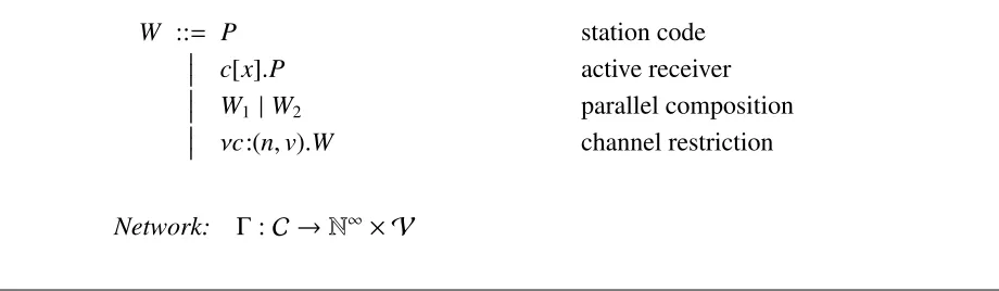
Table 1Wireless systems
W ::= P station code
c[x].P active receiver
W1 |W2 parallel composition
νc:(n,v).W channel restriction
Network: Γ:C →N∞× V
containing the transmission information for channels. A possible evolution of a system will then be given by a sequence of computation steps:
Γ1.W1 _Γ2.W2 _. . . ._Γk.Wk. . . _. . . (1)
where intuitively each step corresponds to either the passage of time, a broadcast from a station, or some unspecified internal computation; the code running at stations evolves as a computation proceeds, but so also does the state of the underlying channel environment. In the following we will use the meta-variableCto range over configurations.
2.1
Syntax
The syntax for configurations is given in Table 1, where P ranges over code for programming individual stations, explained in Table 2. Here c ranges over some set of channel names and v
is an element from some unspecified set of valuesV; all we require of this set is that it contains some error constanterr, which denotes a faulty transmission, and that each valuev(includederr) is associated with a strictly positive integerδv, which denotes the amount of time instants required
by a wireless station to transmit the value.
A system termW is a collection of individual threads running in parallel, with possibly some channels restricted. Note that the definition of the restriction operatorνc:(n,v).W is non-standard, for a restricted channel has a positive integer and a closed value associated; roughly speaking, the termνc:(n,v).W corresponds to the termW where channelcis restricted, and the transmission of valuevover channelcwill take place for the nextninstants of time.
Each thread may be inactive or active, of the formc[x].P, wherexranges over some unspecified set of data-variables; this process represents a wireless station in the process of receiving a value from the channelc. When the value is eventually received the variable xwill be replaced with the received value in the codeP.
Table 2Wireless systems: station code
P,Q ::= c!hui.P broadcast
bc?(x).PcQ receiver with timeout
σ.P delay
τ.P internal activity
P+Q choice
[b]P,Q matching
X process variable
nil termination
fixX.P recursion
σ.P, and broadcast along a channel c!hui.P. Although in principle we could consider a sub-language for data manipulation, for the examples consider in this paper this is unnecessary; so in the broadcast construct ucan be taken to be either a variable xor an actual data value. Of the remaining standard constructs the most notable is matching, [b]P,Qwhich branches toPorQ, de-pending on the value of the Boolean expressionb. We leave the language of Boolean expressions unspecified, other than saying that it should contain equality tests for values,u1 = u2. More
impor-tantly, it should also contain the expression exp(c) for checking if in the current configuration the channelcis exposed, that is it is currently used for transmitting.
In the construct fixX.P occurrences of the recursion variable X in P are bound; similarly in the termsbc?(x).PcQandc[x].Pthe data-variable xis bound inP. This gives rise to the standard notions of free and bound variables,α-conversion and capture-avoiding substitution,{Q/X}Pand
{v/x}P respectively; we ignore the details. We simply assume that all occurrences of variables in
system terms are bound and we will identify systems up toα-conversion. Moreover we assume all occurrences of recursion variables areguarded; they must occur within either a broadcast, input or time delay prefix, or within an execution branch of a matching construct.
We use a number of notational conventions. Q
i∈IWi means the parallel composition of all
systemsWi, fori ∈ I. We identify Qi∈IWi withnilif I = ∅. We will omit trailing occurrences of nil, render νc: (n,v).W asνc.W when the values (n,v) are not relevant to the discussion, and use
νc˜.W as an abbreviation for a sequence ˜cof such restrictions. We writebc?(x).Pcforbc?(x).Pcnil. Finally, we abbreviate the recursive processfixX.bc?(x).PcXwithc?(x).P; as we will see this is a persistent listener at channelcwaiting for an incoming message.
A channel environment is adequately represented as a function from channel names to pairs (n,v) where n ∈ N∞ and v is a value. IntuitivelyΓ(c) = (n,v) means that the network is in the
process of transmitting the valuevalong the channelc, and the transmission will be complete inn
more time units. We will use some suggestive notation for looking up the current state of a channel environment in a network:
• Γ`v c:win place ofΓ(c)=(n,w) for somen.
Intuitively, a channel isexposed when it is currently used for transmitting (at least) a value, that is
Γ`t c:nfor somen> 0. Channel exposure plays a major role in our semantics, and to emphasise
this we use the suggestive notationΓ ` c : exp; the converse, whencis ready for a transmission, will be denoted byΓ ` c : idle. A channel environmentΓis said to be stableifΓ ` c : idlefor every channelc. We also writeΓ≤Γ0ifΓ`
t c:nimpliesΓ0`t c:n0andn≤ n0, for every channel
c.
2.2
Intensional semantics
Our intention is to formally define one computation step of the form Γ1.W1 _ Γ2 .W2. In this
section, we provide an intensional semantics for system terms, where judgements take the form
Γ1 . W1
λ
−−−→ W2. Here λ is an action corresponding to either the broadcast or reception of a
value, time passing or internal activity. Then we show how a computation step of the configuration
Γ1. W1 affects the channel environment, leading toΓ2. Evolutions of channel environments and
system terms in a configuration will be combined in the next section to give computation steps for configurations.
We define our intensional semantics on station code using the following four judgements:
(1) Γ.W −−−−c!→v W0: the systemW broadcasts the valuevalong channelc, resulting in residualW0
(2) Γ.W −−−σ→ W0: the passage of time transforms the systemWintoW0
(3) Γ.W −−→τ W0: an internal action transformsW intoW0
(4) Γ.W −−−−c?→v W0: the effect of the transmission of v along the channel c(by some unknown
entity) transforms W into W0; this relation is used primarily to make the definition of the judgements in (1) more understandable.
In the sequel we useλas a meta-variable ranging over the intensional action labelsτ,c!v,c?vand
σ.
Table 3 contains the rules governing transmission. Rule (Snd) models a non-blocking broadcast of messagev along channelc. A transmission can fire at any time, independently on the state of the network; the notationσδv represents the time delay operatorσ iteratedδ
v times. So when the
processc!hvi.P broadcasts it has to waitδv time units before the residual P is activated. On the
other hand, reception of a message by a time-guarded listenerbc?(x).PcQdepends on the state of the channel environment. If the channelcis free then rule (Rcv) indicates that reception can start and the listener evolves into the active receiverc[x].P.
Table 3Intensional semantics: transmission
(Snd)
Γ.c!hvi.P −−−−c!→v σδv.P (Rcv)
Γ`c:idle
Γ.bc?(x).PcQ −−−−c?→v c[x].P
(RcvFail) Γ
`c:exp
Γ.W −−−−c?→v Γ.W (RcvIgn)
¬rcv(W,c)
Γ.W −−−−c?→v W
(Sync) Γ.W1
c!v
−−−−→ W0
1 Γ.W2
c?v
−−−−→W0
2
Γ.W1 |W2
c!v
−−−−→W10 |W20
(RcvPar) Γ.W1
c?v
−−−−→ W0
1 Γ.W2
c?v
−−−−→W0
2
Γ.W1 |W2
c?v
−−−−→W10 |W20
The rule (RcvIgn) says that if a system can not receive on the channelcthen any transmission along it is ignored. Intuitively, the predicate rcv(W,c) means thatW contains among its parallel components at least one non-guarded receiver of the formbc?(x).PcQwhich is actively awaiting a message. Formally, the predicatercv(W,c) is the least predicate such that
rcv(bc?(x).PcQ,c)=true
rcv(P,c)=true implies rcv(P+Q,c)=true
rcv(Q,c)=true implies rcv(P+Q,c)=true
rcv(P,c)=true implies rcv(fixX.P,c)=true
rcv(W1,c)=true implies rcv(W1 |W2,c)=true
rcv(W2,c)=true implies rcv(W1 |W2,c)=true
rcv(W,c)=true implies rcv(νd.W,c)= true providedd, c
The remaining two rules in Table 3 (Sync) and (RcvPar) serve to synchronise parallel stations on the same transmission [16, 35, 36].
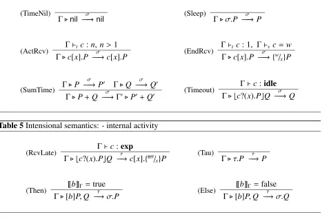
The transitions for modelling the passage of time, Γ. W −−−σ→ W0, are given in Table 4. In the rules (ActRec) and (EndRcv) we see that the active receiver c[x].P continues to wait for the transmitted value to make its way through the network; when the allocated transmission time elapses the value is then delivered and the receiver evolves to {w/x}P. The rule (SumTime) is
necessary to ensuretime determinism. Finally (Timeout) implements the idea thatbc?(x).PcQ is a time-guarded receptor; when time passes it evolves into the alternative Q. However this only happens if the channelcis not exposed. What happens if it is exposed is explained in Table 5.
This table is devoted to internal transitions Γ.W −−→τ W0. Let us first explain rule (RcvLate). Intuitively the process bc?(x).PcQ is ready to start receiving a value on channel c. However ifc
Table 4Intensional semantics: timed transitions
(TimeNil)
Γ.nil −−−σ→ nil (Sleep) Γ. σ.P −−−σ→ P
(ActRcv) Γ`t c:n, n> 1
Γ.c[x].P −−−σ→c[x].P (EndRcv)
Γ`t c: 1, Γ`v c= w
Γ.c[x].P −−−σ→ {w/ x}P
(SumTime) Γ.P σ
−−−→ P0 Γ.Q −−−σ→ Q0
Γ.P+Q −−−σ→Γ0.P0+Q0 (Timeout)
Γ`c:idle
[image:9.612.75.552.97.415.2]Γ.bc?(x).PcQ −−−σ→ Q
Table 5Intensional semantics: - internal activity
(RcvLate) Γ`c:exp
Γ.bc?(x).PcQ −−→τ c[x].{err/
x}P
(Tau)
Γ. τ.P −−→τ P
(Then) ~bΓ =true
Γ.[b]P,Q −−→τ σ.P (Else)
~bΓ=false Γ.[b]P,Q −−→τ σ.Q
the fact that in wireless systems a collision takes place if there is a misalignment between the transmission and reception of a message. The remaining rules are straightforward. Note that in the matching construct we use a channel environment dependent evaluation function for Boolean ex-pressions~bΓ, because of the presence of the exposure predicate exp(c) in the Boolean language.
However checking for the exposure of a channel amounts to listening on the channel for a value. But in wireless systems it is not possible to both listen and transmit within the same time unit, as communication is half-duplex, [38]. As a consequence in our intensional semantics, in the rules (Then) and (Else), the execution of both branches is delayed of one time unit.
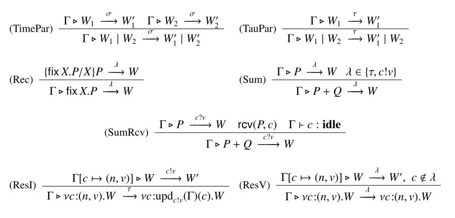
The final set of rules, in Table 6, are structural. In particular (ResI) and (ResV) show how restricted channels are handled. Intuitively moves from the configuration Γ . νc : (n,v).W are inherited from the configurationΓ[c 7→ (n,v)].W; here the channel environmentΓ[c 7→ (n,v)] is the same as Γ except that chas associated with it (temporarily) the information (n,v). However if this move mentions the restricted channel c then the inherited move is rendered as an internal actionτ, (ResI). Moreover the information associated with the restricted channel in the residual is updated, using a function updc!v(·) which is defined later in this section, in Definition 2.4.
Let us provide some results which illustrate the intensional semantics. The first says that trans-missions are non-blocking actions as stations can always synchronise on a transmission at channel
Table 6Intensional semantics: - structural rules
(TimePar) Γ.W1 σ
−−−→W10 Γ.W2
σ −−−→W20
Γ.W1|W2
σ
−−−→W10 |W20 (TauPar)
Γ.W1
τ −−→ W10
Γ.W1 |W2
τ
−−→ W10 |W2
(Rec) {fixX.P/X}P λ −−−→W
Γ.fixX.P −−−→λ W
(Sum) Γ.P λ
−−−→W λ∈ {τ,c!v}
Γ.P+Q −−−→λ W
(SumRcv) Γ.P
c?v
−−−−→W rcv(P,c) Γ`c:idle
Γ.P+Q −−−−c?→v W
(ResI) Γ[c7→(n,v)].W
c!v
−−−−→ W0
Γ. νc:(n,v).W −−→τ νc:updc!v(Γ)(c).W
(ResV) Γ[c7→(n,v)].W λ
−−−→W0, c<λ
Γ. νc:(n,v).W −−−→λ νc:(n,v).W
Lemma 2.1 [Receive enabled] LetΓ.W be a configuration. Then for any channelcand valuev
it holdsΓ.W −−−−c?→v W0for someW0; further
1. ¬rcv(W,c) impliesW0 =W
2. Γ`c:expimpliesW0 =W.
3. rcv(W,c) andΓ`c:idleimpliesW0 , W, and for every valuewΓ.W
c?w
−−−−−→W0.
Proof By transition induction and by inspection of the rules (RcvIgn), (Rcv), (RcvFail) and
(RcvPar).
We can also show that our model of time conforms to a well-established approach in the liter-ature; see for example [35, 47]:
Proposition 2.2
Time determinism: SupposeC −−−σ→ W1andC
σ
−−−→W2. ThenW1 =W2.
Maximal Progress: SupposeC −−−σ→W1. ThenC
λ
−−−9W2, forλ=τ, c!vfor anyc,v,W2.
Proof Both are proved by induction on the derivation ofC −−−σ→ W1.
We end our discussion on the intensional semantics with a technical result on the interaction between stations in systems; this will be useful in later developments.
Proposition 2.3 [Parallel components] LetΓ.W1 |W2be a configuration.
1. Γ.W1 |W2
τ
• either there isW10 such thatΓ.W1
τ
−−→W10 withW = W10 |W2
• or there isW0
2such thatΓ.W2
τ −−→ W0
2withW = W1|W
0
2.
2. Γ . W1 | W2
c?v
−−−−→ W if and only if there are W10 and W20 such that Γ . W1
c?v
−−−−→ W10,
Γ.W2
c?v
−−−−→W0
2andW =W
0
1 |W
0
2.
3. Γ.W1 |W2
c!v
−−−−→W if and only if there areW10 andW20 such that
• Γ.W1
c!v
−−−−→W0
1,Γ.W2
c?v
−−−−→W0
2andW =W
0
1 |W
0
2
• orΓ.W1
c?v
−−−−→W0
1,Γ.W2
c!v
−−−−→ W0
2andW = W
0
1 |W
0
2.
4. Γ.W1 |W2
σ
−−−→ Wif and only if there areW10andW20such thatΓ.W1
σ
−−−→W10,Γ.W2
σ −−−→W20
andW =W10 |W20.
Let us now turn our attention to the evolution of channel environments in a configuration. Here we define a predicate updλ(Γ) which describes how the channel environmentΓchanges when performing the actionλ.
Definition 2.4 [Channel Environment update] LetΓbe an arbitrary channel environment andλan intensional action. We let updλ(Γ) be the unique channel environment determined by the following four definitions:2
updσ(Γ)`t c= (n−1) whenever Γ`t c= n, updσ(Γ)`v c= w whenever Γ`t c= w.
We let updc!v(Γ) be the channel environment such that
updc!v(Γ)`t c=
δv if Γ`c:idle
j if Γ`c:exp updc!v(Γ)`v c=
v if Γ`c:idle
err if Γ`c:exp
whereΓ`t c:kand jis given by max(δv,k). Finally, we let updc?v(Γ)=updc!v(Γ) and updτ(Γ)= Γ.
The definition of updσ(Γ) is straightforward; when time passes, the time of exposure of each channel decreases by one time unit. The predicates updc!v(Γ) and updc?v(Γ) model how collisions are handled in our calculus. When a station begins broadcasting a value v over a channelc this channel becomes exposed for the amount of time required to transmitv, that isδv. If the channel
is not free a collision happens. As a consequence, the value that will be received by a receiving station, when all transmissions over channelcterminate, is the error valueerr. Finally the definition of updτ(Γ) reflects the intuition that internal activities do not affect the exposure state of channels.
2.3
Reduction semantics
We are now in a position to formally define the individual computation steps for wireless systems, alluded to informally in (1) above.
Definition 2.5 [Reduction] We writeΓ.W _Γ0.W0 if
(i) (Transmission)Γ.W −−−−c!→v W0for some channelcand valuev, whereΓ0 =updc!v(Γ)
(ii) (Time)Γ.W −−−σ→W0andΓ0 = upd
σ(Γ)
(iii) or (Internal)Γ.W −−→τ W0andΓ0 =updτ(Γ). The intuition here should be obvious; computation proceeds either by the transmission of values between stations, the passage of time, or internal activity; further, the exposure state of channels is updated according to the performed transition.
Sometimes it will be useful to distinguish between instantaneous reductions and timed reductions; instantaneous reductions,Γ1.W1_i Γ2.W2, are those derived via clauses (i) or (iii) above; timed
reductions are denoted with the symbol_σand coincide with reductions derived using clause (ii).
Example 2.6 [Time-consuming Transmission] Consider a wireless system with two stations, that is a configurationC1of the formΓ1.P1|Q1. Let us suppose
P1 is c!hwi.R, Q1 is bc?(x).ScT1
andΓ1 is a stable channel environment, in thatΓ1 `t d : 0 for all channelsd. Then, assumingδwis
2,
C1 _C2 (2)
whereC2has the formΓ2.P2 |Q2and
P2 is σ2.R Q2 is c[x].S Γ2`t c: 2 Γ2 `v c:w
The move fromP1 toP2is via an application of the rule (Snd), fromQ1toQ2 relies on (Rcv) and
they are combined together using (Sync) to obtainΓ1.P1 |Q1
c!w
−−−−→ P2 |Q2and then the step (2)
results from (Transmission) in Definition 2.5.
The next stepC2 _ C3 is via (Time) in Definition 2.5;C3is of the formΓ3. σ.R | Q2where
the only change to the channel environment is that nowΓ3 `t c: 1. The inference of the transition
Γ2.P2 |Q2
σ
−−−→σ.R | Q2
uses the rules (Sleep), (ActRec) and (TimePar). The final move we consider,C3 _C4 = Γ.R| {w/
x}S, is another instance of (Time). However
steps the valuewhas been transmitted from the first station to the second one along the channelc, in two units of time.
Now suppose we changeP1 toP01 = σ.P1, obtaining thus the configurationC01 = Γ1. P01 | Q1.
Then the first step,C01 _ C02 is a (Time) step, withC02 = Γ1.P1 |T1. Here an instance of the rule
(Timeout) is used in the transition from Q1 to T1. In C02 the station P1 is now ready to transmit
on channel c, but the second station has stopped listening. The next step depends on the exact form ofT1; if for examplercv(T1,c) is false then by an application of rule (RcvIgn) we can derive
C0
2_C
0
3 = Γ2.P2|T1. Here the transmission ofwalongcstarted but nobody was listening.
Finally, supposeT1is a delayed listener on channelc, sayσ.T2whereT2isbc?(y).S2cU2. Then
we have the (Time) step C03 _ C04 = Γ3 . σ.R | T2 and now the second station, T2, is ready to
listen. However, asΓ3 ` c : exp, stationT2 is joining the transmission too late. To reflect this we
can derive we can derive the (Internal) step
C04 _C05 = Γ3. σ.R | c[y].{err/y}S2
using the rules (RcvLate) and (TauPar), amongst others. At the end of the transmission, in one more time step, the second station will therefore end up with an error in reception.
In the revised system C01 = Γ1. σ.P01 | Q1 the second station missed the delayed transmission
from P01. However we can change the code at the second station to accommodate this delay, by replacingQ1 with the persistent listener Q01 = c?(x).S. We leave the reader to check that starting
from the configuration Γ1 . σ.P01 | Q01 the value w will be successfully transmitted between the
stations in four reduction steps.
Example 2.7 [Collisions] Let us now consider a system with three stations,
C1 = Γ.S1 |S2 |R1
where
S1 = σ.c!hv0i
S2 = c!hv1i
R1 = bc?(x).PcT
and Γ is a stable environment; suppose further that δv0 = 1, δv1 = 3. In this configuration the
stationS2 can perform a broadcast, leading to the reductionC1 _ C2 = Γ1.S1 | σ
3 | c[x].P, the
derivation of which requires an instance of the rule (RcvIgn), Γ.S1
c?v1
−−−−−→ S1; here the channel
environmentΓ1is defined as updc!v1(Γ), leading toΓ1(c)= (3,v1). We can now derive the reduction C2_C3 = Γ2.c!hv0i |σ2 |c[x].P, whereΓ2= updσ(Γ1) meaning thatΓ2 `t c: 2.
In this configuration the first station is ready to broadcast a value v0 along channel c. Since
there is already a value being transmitted along this channel, we expect this second broadcast to cause a collision; further, since the amount of time required for transmitting valuev0is shorter than
that needed to end the transmission of valuev1, we expect that the broadcast performed by the first
Formally this is reflected in the reductionC3 _ C03 = Γ02. σ |σ2 |c[x].P. Here the reduction of the system term uses the sub-inferenceΓ2. σ2 |c[x].P
c?v1
−−−−−→σ2 |c[x].P, which can be derived using either rules(RcvFail), (RcvIgn). ConsequentlyΓ0
2 = updc!v0(Γ2), and sinceΓ2 ` c : expwe
obtainΓ0
2(c) = (2,err); this represents the fact that a collision has occurred, and thus the special
valueerrwill eventually be delivered onc. At this point we can derive the reductions C0
3 _σ_σ C4 = Γ.nil | nil | {err/x}P, meaning
that the transmission along channelcterminates in 2 time instants, leading the receiving station to detect a collision each of the two transitions above can be inferred using the rules in Table 4.
Now, suppose we change the amount of time required to transmit value v0 from 1 to 3, and
consider again the configurationC3above. In this case the transmission of valuev0will also cause
a collision; however, in this case the transmission of valuev0 is long enough to continue after that
of value v1 has finished; as a consequence, we expect that the time required for channel cto be
released rises when the broadcast ofv0happens.
In fact, in this case we have the reduction C3 _ C003 = Γ002 . σ3 | σ2 | c[x].P, where
Γ00
2 =updc!v0(Γ2) and specificallyΓ
00
2(c)= (3,err). Now, three time instants are needed for the
trans-mission along channelcto end, leading to the sequence of (timed) reductionsC00
3 _σ_σ_σ C4.
2.4
Behavioural semantics
In this section we propose a notion of timed behavioural equivalence for our wireless networks. Our touchstone system equality isreduction barbed congruence[19, 42, 30, 21], a standard con-textually defined process equivalence. Intuitively, two terms are reduction barbed congruent if they have the same basic observables, in all parallel contexts, under all possible computations. The formal definition relies on two crucial concepts, a reduction semantics to describe how sys-tems evolve, which we have already defined, and a notion of basic observable which says what the environment can observe directly of a system. There is some choice as to what to take as a basic observation, or barb, of a wireless system. In standard process calculi this is usually taken to be the ability of the environment to receive a value along a channel. But the series of examples we have just seen demonstrates that this problematic, in the presence of possible collisions and the passage of time. Instead we choose a more appropriate notion for wireless systems, one which is already present in our language for station code.
Definition 2.8 [Barbs] We say the configurationΓ.Whas astrong barb on c, writtenΓ.W ↓c, if
Γ`c:exp. We writeΓ.W ⇓c, aweak barb, if there exists a configurationC0such thatΓ.W _∗C0
andC0 ↓c. Note that we allow the passage of time in this definition of weak barbs.
Definition 2.9 LetRbe a relation over well-formed configurations.
(1) Ris said to bebarb preservingifΓ1.W1⇓c impliesΓ2.W2 ⇓c, whenever (Γ1.W1)R (Γ2.W2).
(2) It is reduction-closed if (Γ1 .W1) R (Γ2 .W2) andΓ1 .W1 _ Γ
0
1. W
0
1 imply there is some
Γ0
2.W
0
2such thatΓ2.W2 _
∗ Γ0
2.W
0
2and (Γ
0
1.W
0
1)R (Γ
0
2.W
0
(3) It iscontextualifΓ1.W1 R Γ2.W2, impliesΓ1.(W1 |W) R Γ2.(W2|W) for all processes
W.
With these concepts we now have everything in place for a standard definition of contextual equiv-alence between systems:
Definition 2.10 [Reduction barbed congruence], written', is the largest symmetric relation over configurations which is barb preserving, reduction-closed and contextual.
In the remainder of this section we explore via examples the implications of Definition 2.10. The notion of a fresh channel will be important; we say thatcisfreshfor the configurationΓ.W
if it does not occur free inW andΓ` c:idle. Note that we can always pick a fresh channel for an arbitrary configuration.
Example 2.11 Let us assume thatΓ` c:idle. Then it is easy to see that
Γ.c!hvoi.P ; Γ.c!hv1i.P (3)
under the assumption thatvoandv1are different values. For letT be the testing context
bc?(x).[x= vo]eureka!hoki,nilc
whereeurekais fresh, andok is some arbitrary value. ThenΓ.c!hvoi.P | T has a weak barb on
eurekawhich is not the case for Γ.c!hv1i.P | T. Since'is contextual and barb preserving, (3)
above follows.
However such tests will not distinguish between
Q1= c!hvoi |c!hv1i.P and Q2 =c!hv1i |c!hv0i.P
under the assumption that δv0 = δv1. In both configurations Γ. Q1 and Γ. Q2 a collision will
occur at channelcand a third station, such asT, will receive the error valueerrat the end of the transmission. So there is reason to hope thatΓ.Q1 ' Γ.Q2.However we must wait for the next
section for proof techniques for establishing such equivalences; see Example 3.4.
The above example suggests that transmitted values can be observed only at the end of a trans-mission; so if a collision happens, there is no possibility of determining the value that was origi-nally broadcast. This concept is stressed even more in the following example.
Example 2.12 [Equating values] LetΓbe a stable channel environment,W0 =c!hv0i,W1 =c!hv1i
and consider the configurationsΓ.W0,Γ.W1; here we assume thatv0andv1are two different values
with possibly different transmission times.
We already argued in Example 2.11 that these two configurations can be distinguished by the context
However, the two configurations above can be made indistinguishable if we add to each of them a parallel component that causes a collision on channelc. To this end, let
Eq(v0,v1)= σh.c!hoki
for some positive integerhand valueok such thath < min (δv0, δv1) andδok ≥ max (δv0, δv1)− h.
Now, consider the configurationsC0= Γ.W0 |Eq(v0,v1),C1 = Γ.W1 |Eq(v0,v1).
One could hope that there exists a context which is able to distinguish these two configurations. However, before the transmission of v0 ends in C0, a second broadcast along channel cwill fire,
causing a collision; the same happens before the end of transmission of valuev1inC1. Further, the
total amount of time for which channelc will be exposed is the same for both configurations, so that one can argue that it is impossible to provide a context which is able to distinguishC0 from
C1. In order to prove this to be formally true, we have to wait until the next section. Collisions can also be used to merge two different transmissions on the same channel in a single corrupted transmission.
Example 2.13 [Merging Transmissions] LetΓbe a stable channel environment,
W0 = c!hv0i.c!hv1i, W1 = c!hv1i.c!hv0i. InΓ. W0 a broadcast of value v0 along channel c can
fire; when the transmission ofv0is finished, a second broadcast of valuev1along the same channel
can fire. The behaviour ofΓ.W1 is similar, though the order of the two values to be broadcast is
swapped. Note that it is possible to distinguish the two configurationsΓ.W0andΓ.W1using the
test
bc?(x).[x= vo]eureka!hoki,nilc
we have already seen in the previous example.
However suppose now that we add a parallel component to both configurations which broad-casts another value along channelcbefore the transmission of valuev0(v1) has finished, and which
terminates after the broadcast of valuev1 (v0) has begun. More formally, let
Mrg(v0,v1)=σh.c!hoki
whereh= min(δv0, δv1)−1 andδok= |δv0 −δv1|+2.
Consider the configurationsΓ.W0| Mrg(v0,v1),Γ.W1 | Mrg(v0,v1). In both configurations a
collision occurs; further, once the transmission of valuev0has begun in the former configuration,
channelcwill remain exposed until the transmission of valuev1has finished. A similar behaviour
can be observed on the second configuration. This leads to the intuition thatΓ.W0| Mrg(v0,v1)'
Γ0.W
1 | Mrg(v0,v1); we prove this in Example 3.6, for a particular instance of transmission values
forv0,v1.
Example 2.14 [Observing the passage of time] Consider the two processes Q1 = c!hvoi and
Q2 = σ.Q1, and again let us assume that Γ ` c : idle. There is very little difference between
the behaviours of Γ.Q1 andΓ. Q2; both will transmit (successfully) the value vo, although the
latter is a little slower. However this slight difference can be observed. Consider the testT defined by
[exp(c)]eureka!hoki,nil
In fact,Γ.(Q1 |T) can start a transmission along channelc, after which the predicate exp(c) will
be evaluated in the system termT. The resulting configuration is given byΓ0.σδv0 |σ.eureka!hoki;
at this point, it is not difficult to note that the configuration has a weak barb oneureka.
On the other hand, the unique reduction fromC2 = Γ.(Q2 |T) leads to the evaluation of the
exposure predicate exp(c); sinceΓ ` c : idlethe only possibility for the resulting configuration is given byC02 = Γ.Q2 |σ. Sinceeurekais a fresh channel, it is now immediate to note thatC02 6⇓eureka.
For the test to work correctly it is essential that Γ ` c : idle; using the proof methodology developed in Section 3.2 we are able to show that ifΓ0 `
t c:nandn> δv0 thenΓ
0.Q
1 'Γ0.Q2.
Behind this example is the general principle that reduction barbed congruence is actually sen-sitive to the passage of time; this is proved formally in Proposition 4.17 of Section 4.3.
Example 2.15 As a final example we illustrate the use of channel restriction. Assume thatv1and
v2are some kind of comparable values. Consider the configuration
Γ. νc: (0,·).(c!hv1i | Pe |R) where the station code is given by
Pe =σ.fixX.([exp(c)]X,c!hv2i)
R=c?(x).R1
R1 =c?(y).[x> y]d!hxi,d!hyi
Intuitively the receiverRwaits indefinitely for two values along the restricted channelcand broad-casts the largest on channeld. Intuitively the use of channel restriction here shelterscfrom external interference. AssumingΓ`d :idlewe will be able to show that
Γ. νc: (0,·).(c!hv1i.nil|Pe |R) ' Γ. σδv1+δv2+2.d!hwi.nil
providedw=max(v1,v2).
We end this section with a small technical result, which will be extremely useful in the de-velopment of our behavioural theory. Informally it says that internal reductions do not affect the remaining delivery time of values.
Lemma 2.16 WheneverΓ.W _∗i Γ0.W0it holds thatΓ≤ Γ0.
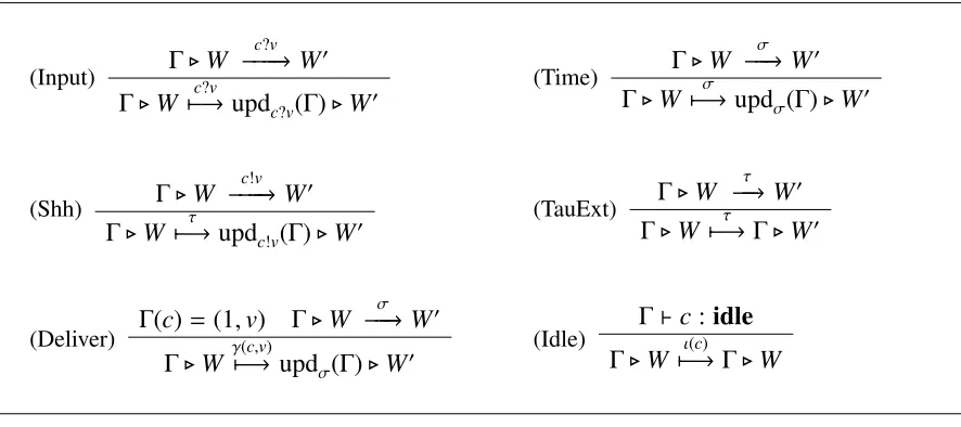
Table 7Extensional actions
(Input) Γ.W
c?v
−−−−→ W0
Γ.W 7−→c?v updc?v(Γ).W
0 (Time)
Γ.W −−−σ→ W0
Γ.W 7−→σ updσ(Γ).W0
(Shh) Γ.W
c!v
−−−−→W0
Γ.W 7−→τ updc!v(Γ).W0
(TauExt) Γ.W τ −−→W0
Γ.W 7−→τ Γ.W0
(Deliver) Γ(c)=(1,v) Γ.W σ −−−→ W0
Γ.W γ7−→(c,v)updσ(Γ).W0
(Idle) Γ
`c:idle
Γ.W 7−→ι(c) Γ.W
3
Extensional Semantics
The intention here is to give a co-inductive characterisation of the contextual equivalence'
between configurations, in terms of a standard bisimulation equivalence over some extensional LTS. First, we present the extensional semantics, then we recall the standard definition of (weak) bisimulation over configurations; finally its usefulness is illustrated by means of a number of ex-amples.
3.1
Extensional actions
The question here is what activity of a wireless system is observable externally? Example 2.14 indicates that the passage of time is observable. From Lemma 2.1, we know that all systems are always ready to receive transmissions, that is are input-enabled, but we will have to take into account the effect of these inputs. In contrast the discussion in Example 2.11 indicates that, due to the possibility of collisions, the treatment of transmissions is more subtle. It turns out that the transmission itself is not important; instead we must take into consideration the successful delivery of the transmitted value.
In Table 7 we give the rules defining the extensional actions,C 7−→ Cα 0, which can take one of the forms:
• Input:C7−→ Cc?v 0. This is inherited directly from the intensional semantics.
• Time: C7−→ Cσ 0, also inherited from the intensional semantics.
• Internal: C 7−→ Cτ 0. This corresponds to the combination of the Internal and Transmission
rules from the reduction semantics, in Definition 2.5.
• Delivery: Cγ7−→ C(c,v) 0. This corresponds to the successful delivery of the value
• Free: C 7−→ Cι(c) , a predicate indicating that channel cis not exposed, and therefore ready to start a potentially successful transmission.
3.2
Bisimulation equivalence
The extensional actions of the previous section endows systems in CCCP with the structure of an
LTS. Weak extensional actions in this LTS are defined as usual, with C =⇒ Cα 0 denoting C 7−→τ ∗
α
7−→7−→τ ∗ C0. We will useC
=⇒ C0 to denoteC 7−→τ ∗ C0, and the formulation of bisimulations is
facilitated by the notationC=⇒ Cαˆ 0, which is again standard: forα=τthis denotesC=⇒ C0while forα,τit isC=α⇒ C0. We now have the standard definition of weak bisimulation equivalence in
the resulting LTS which for convenience we recall.
Definition 3.1 LetRbe a binary relation over configurations. We say that Ris a bisimulation if for every extensional actionα, wheneverC1 R C2
(i) C1 7−→ Cα 0
1impliesC2 ˆ
α
=⇒ C0
2, for someC
0
2, satisfyingC
0
1 R C
0
2
(ii) conversely,C27−→ Cα 0
2impliesC1 ˆ
α
=⇒ C0
1, for someC
0
1, such thatC
0
1 R C
0
2.
We writeC1 ≈ C2, if there is a bisimulationRsuch thatC1 R C2.
Our goal is to demonstrate that this form of bisimulation provides a sound and useful proof method for showing behavioural equivalence between wireless systems described in CCCP; moreover for a large class of systems it will also turn out to be complete. But our first examples show that the introduction of the actionsι(c) andγ(c,v) are necessary for soundness.
Example 3.2 [On the rule (Idle)] Suppose we were to drop the rule (Idle) in the extensional se-mantics; then consider the configurations
Γ1.W1 = τ.nil
Γ2.W2 = c!hvi
whereΓ1(c)=(1,v),Γ2(c)= (0,·) andδv =1.
If we were to drop the actions ι(c) from the extensional semantics then the extensional LTS generated by these two configurations would be isomorphic; recall that an output action in the intensional semantics always corresponds to a τaction in its extensional counterpart. Thus they would be related by the amended version of bisimulation equivalence.
However, we also have thatΓ1.W1; Γ2.W2. This can be proved by exhibiting a distinguishing
context. To this end, consider the systemT =[exp(c)]nil,eureka!hoki. ThenΓ2.W2 |T has a weak
Example 3.3 [On the rule(Deliver)] Consider the configuration
Γ2.W3 =c!hwi
where δw = 1 and Γ2 is as in the previous example, and the testing context T0 = c(x).[x =
v]eureka!hoki,nil. Then, assuming w is different from v, Γ2 . W3 | T0 can not produce a barb
on eureka.
However ifW2 is the code c!hvi, as in the previous example, then obviouslyΓ2 .W3 | T0 can
produce such a barb. It follows thatΓ2.W2 ;Γ2.W3.
Now if we were to drop the rule(Deliver)in the extensional semantics, thereby eliminating the actions γ(c,v), then it would be straightforward to exhibit a bisimulation containing this pair of configurations. Thus again the amended version of bisimulation equivalence would be unsound.
The two examples above show that both rules (Idle)and(Deliver) are necessary to achieve the soundness of our bisimulation proof method for reduction barbed congruence. In the remainder of this section we give a further series of examples, showing that bisimulations in our extensional LTS offers a viable proof technique for demonstrating behavioural equivalence for at least simple wireless systems.
Example 3.4 [Transmission] Here we revisit Example 2.11. Let Γbe a stable channel environ-ment, and consider the configurations C0 = Γ . W, C1 = Γ . V, where W = c!hv0i.P|c!hv1i,
V = c!hv1i.P|c!hv0i; note these two configurations are taken from the second part of in Example
2.11.
Our aim is to show thatC0 ≈ C1, and for convenience let us we assume thatδv0 = δv1 = 1. The
idea here is to describe the required bisimulation by matching up system terms. To this end we define the following system terms:
W0 = σ.P|c!hv1i V1 = σ.P|c!hv0i
W1 = c!hv0i.P|σ V0 = c!hv1i.P|σ
E = σ.P|σ E0 = P|nil
Then for any channel environment∆we have the following transitions in the extensional semantics:
∆.W 7−→τ updc!v0(∆).W0 ∆.V τ
7−→ updc!v0(∆).V0
∆.W 7−→τ updc!v
1(∆).W1 ∆.V
τ
7−→ updc!v
1(∆).V1
∆.W 7−→d?w updd?w(∆).W ∆.V 7−→d?w updd?w(∆).V
∆.W 7−→ι(d) ∆.W if∆`d:idle ∆.V 7−→ι(d) ∆.V if∆`d :idle
∆.W0
τ
7−→ updc!v1(∆).E ∆.V0
τ
7−→ updc!v1(∆).E
∆.W0
d?w
7−→ updd?w(∆).W0 ∆.V0
d?w
7−→ updd?w(∆).V0
∆.W0
ι(d)
7−→ ∆.W0if∆`d :idle ∆.V0
ι(d)
Table 8A relationSfor comparing the configurationsC0,C1of Example 3.5
∆.W S ∆.V
∆.W0 S ∆.V0
(∆[c7→(1,v0)]).W0 S (∆[c7→ (2,v1)]).V1
(∆[c7→ (1,err)]).W0 S (∆[c7→ (2,err)]).V1
Λ.Wok S Λ.Vok
∆.Werr S ∆.Verr
∆.W0 S ∆.V0
∆arbitrary channel environment,
Λarbitrary channel environment such thatΛ(c)=(k,w) for somek≥ 2
∆.W1
τ
7−→ updc!v0(∆).E ∆.V1
τ
7−→ updc!v0(∆).E
∆.W1
d?w
7−→ updd?w(∆).W1 ∆.V1
d?w
7−→ updd?w(∆).V1
∆.W1
ι(d)
7−→ ∆.W1if∆`d :idle ∆.V1
ι(d)
7−→ ∆.V1if∆`d :idle
Heredranges over arbitrary channel names, includingc. Then consider the following relation:
S= {(∆.W,∆.V), (∆.W0, ∆.V0),(∆.W1,∆.V1) | ∆is a channel environment}
Using the above tabulation of actions one can now show thatSis astrongbisimulation; forC S C0
each possible action ofCcan be matched byC0by performing exactly the same action, and vice-versa.
Since (C0,C1)∈ S, it follows thatC0≈ C1.
Example 3.5 [Equators] Let us consider again the configurationsC0,C1of Example 2.12. Recall that C0 = Γ.W, where W = c!hv0i | σh.c!hokiandC1 = Γ. V, where V = c!hv1i | σh.c!hoki;
further, recall that Γis a stable channel environment andh,okare a positive integer and a value, respectively, such that h < min (δv0, δv1), δok ≥ max (δv0, δv1)−h. Without loss of generality, for
this example we assumeδv0 =1, δv1 =2,h= 0 andδok =2.
For the sake of convenience we define the following system terms:
W0 = σ|c!hoki V1 = σ2|c!hoki
Wok = c!hv0i |σ2 Vok = c!hv1i |σ2
Werr = σ|σ2 Verr = σ2|σ2 W0 = nil|σ V0 = σ|σ
E = nil|nil
Let us consider the relationS depicted in Table 8; note that (C0,C1) ∈ S, so that in order to prove thatC0 ≈ C1 it is sufficient to show thatSis a bisimulation. Note that in the relationSthe
system termsWok,Vokare always associated with a channel environment in which the channelcis
to prove thatΛ.Werr 0 Λ.Verr; this is because the values broadcast by these two configurations
are different.
Let us list the main the extensional actions from configurations using these system terms:
∆.W 7−→τ (∆[c7→(1,v0)]).W0if∆`c:idle
∆.V 7−→τ (∆[c7→(2,v1)]).V1if∆`c:idle
∆.W 7−→τ (∆[c7→(2,ok)]).Wok
∆.V 7−→τ (∆[c7→(2,ok)]).Vok
∆.W 7−→d?w (updd?w(∆)).W
∆.V 7−→d?w (updd?w(∆)).V
(∆[c7→(1,v0)]).W0
τ
7−→ (∆[c7→(2,err)]).Werr
(∆[c7→(2,v1)]).V1
τ
7−→ (∆[c7→(2,err)]).Werr
∆.W0
c?w
7−→ (∆[c7→(1,err)]).W0if∆` c:exp, δw =1
∆.V1
c?w
7−→ (∆[c7→(2,err)]).V1if∆` c:exp, δw =1
∆.W0
c?w
7−→ (∆[c7→(δw,err)]).W0if∆` c:exp, δw >1
∆.V1
c?w
7−→ (∆[c7→(δw,err)]).V1if∆` c:exp, δw >1
Λ.Wok
τ
7−→ (updc!v0(Λ)).Werr
Λ.Vok
τ
7−→ (updc!v
1(Λ)).Verr
∆.Werr 7−→σ (updσ(∆)).W0
∆.Verr
σ
7−→ (updσ(∆)).V0
∆.W0 7−→σ (updσ(∆)).E
∆.V0 7−→σ (upd
σ(∆)).E
Here∆,Λ are two arbitrary channel environments, but Λ is subject to the constraint that Λ(c) = (k,w) for some value w and integer k ≥ 2. Note that in this case we have that (updc!v0(Λ)) =
(updc!v
1(Λ)). With the aid of this tabulation one can now show thatSis indeed a bisimulation and
therefore thatC0 ≈ C1.
Example 3.6 [Merging] The last example we provide considers the merging of two transmissions in a single transmission. LetΓbe a stable channel environment andv0,v1 be two values such that
δv0 =1, δv1 =2. Also letokbe a value such thatδok = 3. Consider the configurations
C0 = Γ.W C1 = Γ.V
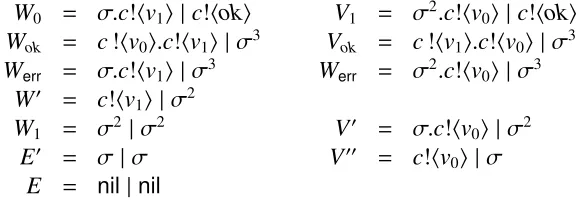
Table 9A relationSfor comparing the configurationsC0,C1of Example 3.6
∆0.W S ∆0.V
∆1.W0 S ∆2.V1
∆3.Wok S ∆3.Vok
∆3.Werr S ∆3.Verr
∆2.W0 S ∆2.V0
∆2.W1 S ∆2.V0
∆1.E0 S ∆1.V00
∆n,n≥0 arbitrary channel environment such that∆`t c:mfor some integerm≥ n.
ThenC0 ≈ C1. As in previous examples, this statement can be proved formally by exhibiting a bisimulation that contains the pair (C0,C1); to this end, define the following system terms:
W0 = σ.c!hv1i |c!hoki V1 = σ2.c!hv0i |c!hoki
Wok = c!hv0i.c!hv1i |σ3 Vok = c!hv1i.c!hv0i |σ3
Werr = σ.c!hv1i |σ3 Werr = σ2.c!hv0i |σ3
W0 = c!hv
1i |σ2
W1 = σ2|σ2 V0 = σ.c!hv0i |σ2
E0 = σ |σ V00 = c!hv0i |σ
E = nil|nil
Consider now the relationSdepicted in Table 9; note thatC0 S C1. We leave the reader to check thatSis also a weak bisimulation, from whichC0≈ C1follows.
4
Full abstraction
In this section, we show that the co-inductive proof method based on the bisimulation of the pre-vious section is both sound respect to the contextual equivalence of Section 2.4; this is the subject of Section 4.1. Moreover it is complete for a large class of systems. This class is isolated in the following section, and the completeness result is then given in Section 4.3.
4.1
Soundness
In this section we prove that (weak) bisimulation equivalence is contained in reduction barbed congruence. The main difficulty is in proving the contextuality the bisimulation equivalence. But first some auxiliary results.
Lemma 4.1 [Update of Channel Environments] IfΓ.W =⇒Γ0.W0thenΓ≤Γ0.
Corollary 4.2 For any channelc,Γ.W =ι(⇒c) impliesΓ.W 7−→ι(c). Corollary 4.2 is very useful when proving that the exposure state of channels is preserved by bisimilar configurations.
Below we report a result on channel exposure for bisimilarity; a similar result for reduction barbed congruence will also be proved, in Proposition 4.14.
Lemma 4.3 [Channel exposure wrt≈] WheneverΓ1.W1≈ Γ2.W2thenΓ1 `c:idleif and only
ifΓ2 `c:idle.
Proof SupposeΓ1.W1 ≈Γ2.W2. IfΓ1 `c :idlethen by definition of Rule(Idle)of Table 7 it
follows thatΓ1.W1
ι(c)
7−→. AsΓ1.W1 ≈Γ2.W2, it follows thatΓ2.W2
ι(c)
=⇒. From Corollary 4.2 we have thatΓ2.W2
ι(c)
7−→, and by the definition of Rule(Idle)thatΓ2 `c:idle.
In order to prove that weak bisimulation is sound with respect to reduction barbed congruence we need to show that≈is preserved by parallel composition.
Theorem 4.4 [≈is contextual] SupposeΓ1.W1 ≈Γ2.W2. Then for any system termW,Γ1.(W1|
W)≈ Γ2.(W2|W).
Proof Let the relationSover configurations be defined as follows:
{ Γ1.W1 |W, Γ2.W2 |W) : Γ1.W1 ≈ Γ2.W2}
It is sufficient to show thatSis a bisimulation in the extensional semantics. To do so, by symmetry, we need to show that an arbitrary extensional action
Γ1.W1 |W
α
7−→Γb1.Wc1 (4)
can be matched byΓ1.W2|W via a corresponding weak extensional action.
The action (4) can be inferred by any of the six rules in Table 7. We consider only one case, the
most difficult one(Shh). So hereαisτandΓ1.W1 |W
c!v
−−−−→Wc1, for somecandv. This transition
in turn can always be inferred by an application of the rule (Sync)from Table 3. Without loss of generality we can assume
• Γ1.W1
c!v
−−−−→ W10 • Γ1.W −−−−c?→v W0
• Wc1 =W10 |W0
By an application of rule(Shh)it follows thatΓ1.W1
τ
7−→Γ01.W10, withΓ01 =updc!v(Γ1). Since
Γ1.W1 ≈Γ2.W2, there isΓ02.W20such thatΓ2.W2 = ⇒ Γ02.W20 andΓ01.W10 ≈Γ02.W20. Now, there
1. LetΓ1` c:exp. By Lemma 2.1(2), in the transitionΓ1.W
c?v
−−−−→W0it must be thatW0 =W. SinceΓ1.W1 ≈Γ2.W2andΓ01.W10 ≈Γ02.W20, by two applications of Lemma 4.3 it follows
that:
• for any channeld,Γ1` d:idleiff Γ2` d:idle
• for any channeld,Γ01` d:idleiff Γ02` d:idle. We recall thatΓ0
1 = updc!v(Γ1), and henceΓ01 andΓ1 may only differ for the entry at channel
c. As a consequence, alsoΓ2andΓ02may only differ for the same entry.
Now, let us analyse the transitions which constitute the weak derivation
Γ2.W2 =⇒Γ02.W
0
2
In particular, let
Γ2.W2=⇒Γn2.W
n
2
τ
7−→Γn2+1.W2n+1 =⇒Γ02.W
0
2 .
There are two possibilities.
(a) Γn
2.W
n
2
τ 7−→Γn+1
2 .W
n+1
2 is derived by an application of rule(TauExt)becauseΓ
n
2.W
n
2
τ −−→ W2n+1. This case is easy.
(b) Γn
2.W
n
2
τ 7−→Γn+1
2 .W
n+1
2 is derived by an application of rule(Shh)becauseΓ
n
2.W
n
2
d!w
−−−−→ W2n+1, for some d and w. Since Γ2 and Γ02 may only differ for the entry at channel c,
also Γn
2 and Γ
n+1
2 may only differ for the same entry. This is because the derivation
Γ2 . W2 =⇒ Γ02 .W20 is untimed, and once a channel becomes exposed it remains so
for the whole derivation. By Lemma 4.3, Γ1 ` c : exp implies Γ2 ` c : exp. By
definition of rule(Shh),Γn+1
2 ` d:exp. Since only the entry atcmay change during the
derivation it follows thatΓn
2 `d :exp(also ford= c). By Lemma 2.1(2), this implies
Γn
2 .W
d?w
−−−−−→W. By an application of rule (Sync)and one application of rule(Shh) we can derive
Γn
2.W
n
2 |W
τ
7−→Γn2+1.W2n+1 |W
As a consequence,
Γ2.W2|W =⇒Γ02.W
0
2 |W
with Γ01.W10 |W, Γ02.W20 |W∈ S
.
2. LetΓ1 `c:idle. There are two sub-cases.
(a) Let¬rcv(W,c). This case is similar to case 1. In fact, by Lemma 2.1(1) the systemWis not affected by the transmission atc. More precisely, the transitionΓ1.W1 |W
c!v
−−−−→Wc1
can only be derived by an application of rule(Sync)because
• Γ1.W1
c!v
• Γ1.W −−−−c?→v W • Wc1 =W10 |W.
(b) Letrcv(W,c). By Lemma 2.1(3) the transition Γ1. W
c?v
−−−−→ W0 must haveW0
, W.
SinceΓ1.W1 ≈Γ2.W2, by Lemma 4.3 it follows thatΓ2` c:idle. AsΓ01= updc!v(Γ1),
it follows that Γ01 ` c : exp. Since Γ01.W10 ≈ Γ0
2. W
0
2, by Lemma 4.3 it follows that
Γ0
2 ` c : exp. As a consequence, the derivationΓ2 .W2 =⇒ Γ
0
2 . W
0
2 must contain a
transition which changes the exposure state of channelc. More precisely, the derivation must have the form
Γ2.W2=⇒Γn2.W
n
2
τ
7−→Γn2+1.W2n+1 =⇒Γ02.W20
where the transition Γn
2 . W
n
2
τ 7−→ Γn+1
2 . W
n+1
2 is due to an application of rule (Shh)
becauseΓn
2. W
n
2
c!w
−−−−→ Wn+1
2 , for some w, with Γ
n
2 ` c : idleand Γ
n+1
2 ` c : exp. By
Lemma 2.1(3) it follows thatΓn2 .W −−−−−c?w→ W0, for any w. By an application of rule
(Sync)and one of rule(Shh), it follows that
Γn
2.W
n
2 |W
τ
7−→Γn2+1.W2n+1 |W0
For any other transition in the derivationΓ2.W2 =⇒ Γ02. W
0
2 we can apply the same
reasoning as in case 1. In particular, for those transitions which are derived by an application of rule(Shh) because of a transition labelled d!w0, the channeld must be
exposed before and (obviously) after the transition. So, by Lemma 2.1(2) the systems
W and W0 can perform the corresponding action d?w0 remaining unchanged. More precisely, we have
Γ2.W2 |W =⇒Γn2.W
n
2 |W
τ
7−→Γn2+1.W2n+1 |W0 =⇒τ Γ02.W20 |W0
with Γ01.W10 |W0, Γ02.W20 |W0∈ S
.
Theorem 4.5 [Soundness]C1 ≈ C2impliesC1 ' C2.
Proof It suffices to prove that bisimilarity is reduction-closed, barb preserving and contextual. Reduction closure follows from the definition of bisimulation equivalence. The preservation of barbs follows directly from Lemma 4.3. Contextuality follows from Theorem 4.4.
4.2
Well-formed systems
reception; this would be necessary, for example, if we wished to investigate the behaviour of its residual after the actionc?v.
LetTc,v denote the systemc!hvi.eureka!hoki+fail!hnoi, whereeurekaandfailare some fresh
channels. Then intuitively we might expect that, at least informally,Γ.Wwill have performed the actionc?vwhen the combined system Γ.(W | Tc,v) no longer has a barb onfailbut does have a
barb oneureka.
However the existence of the barb on eureka depends on the ability of time to pass in the combined system: the transmission alongccan commence, but the delivery ofvtakes time. If time can not proceed then the potential barb oneurekawill never materialise.
Example 4.6 LetW denote the systemd[x].P, for some channelddifferent fromc, and suppose
Γ` d :idle. ThenΓ.(W |Tc,v) can never produce a barb oneureka: Γ.(W |Tc,v)_
∗ C0
implies
C0↓
eureka is not true.
Note in particular that the sub-configuration Γ. W can not perform a σ action; it does not allow time to pass. The only possible rule that might be applied is(EndRcv)from Table 4; but this requiresΓ`t d:nfor somen> 1, whereasΓ`d :idle.
Definition 4.7 [Well-formedness] The set of well-formed configurations WNets is the least set such that
Γ.P∈WNets for all processesP
Γ` c:exp implies Γ.c[x].P∈WNets
Γ.W1,Γ.W2∈WNets implies Γ.W1|W2 ∈WNets
Γ[c7→(n,v)].W ∈WNets implies Γ. νc: (n,v).W ∈WNets
Intuitively a configurationΓ.W is well-formed if it does not contain any receiving station along an idle channel. Note that the configuration used in Example 4.6 is not well-formed.
Lemma 4.8 SupposeCis well-formed andC_C0
. ThenC0
is also well-formed.
Proof SupposeΓ.W −−−→λ W0andΓ.W. Then by rule induction onΓ.W −−−→λ W0one can show that updλ(Γ).W0is also well-formed.
The result now follows by consideration of the three possible cases for deriving C _ C0 in
Definition 2.5.
The main property of well-formed systems is that they allow the passage of time, so long as all internal activity has ceased:
Proposition 4.9 LetΓ.W be a well-formed configuration such thatΓ.W 6_i; thenΓ.W _σ.
It would seem that restricting attention to well-formed configurations does not preclude the phenomenon exhibited in Example 4.6 from occurring. Since our language for station code in-cludes recursion the reader could argue that it is possible to write systems which can perform an infinite sequence of instantaneous reductions; we first identify this systems formally, then we show that these cannot be obtained in our calculus.
Example 4.10 Let W denote the code fixX.τ.X. Then we have an infinite sequence of internal actions
Γ.W _i C1_i . . .Ck _i
Indeed one can show that ifΓ.W _∗ C0 thenC0
_i. Maximal progress then ensures thatC
0 6
_σ.
Definition 4.11 [Well-timed configurations] A configurationCiswell-timed, [27], if there exists an upper boundk∈Nsuch that wheneverC_h
i C
0 for someh≥ 0, thenh≤k.
While well-formedness is a simple syntactic constraint, well-timed means that the designer of the network has to ensure that the code placed at the station nodes can never lead to divergent behaviour. One simple method for ensuring this is to only use recursive definitionsfixX.Pwhere
X is weakly guarded in P; that is, every occurrence of X is within an input, output or time delay prefix, or it is included within a branch of a matching construct. These are exactly the conditions that we placed for recursion variables when defining our calculus. Thus, we would expect every configuration in our calculus to be well-timed. In order to prove formally this statement, we need the following technical result:
Proposition 4.12 An environmentρis a partial mapping from process variables to closed terms. Given a termWand an environmentρ, we denote withWρthe system term obtained by substituting each free occurrence of any process variableXwithρ(X), if defined.
For any channel environmentΓ, (possibly open) termW and environmentρsuch thatΓ.Wρis well-defined then it is also well-timed.
Proof By structural induction on the termW, using the hypothesis that we only allow guarded
recursion.
Corollary 4.13 Any well-formed configurationΓ.W is also well-timed.
Proof Note that ifΓ.Wis well-formed thenWis closed by definition. Thus, for any environment
To end this section we prove a very useful result for well-defined configurations; the proof emphasises the roles of well-formedness and well-timedness in the configurations being tested.
Proposition 4.14 Suppose Γ1.W1 ' Γ2 .W2, where both are well-formed. ThenΓ1 ` c : idle
impliesΓ2 `c:idle.
Proof LetΓ1.W1' Γ2.W2and supposeΓ1 `c :idlefor some channelc. Consider the testing
code:
T =[exp(c)]nil,eureka!hoki
From the definition of 'we know thatΓ1 .W1 | T ' Γ2. W2 | T. SinceΓ1 .W1 is well-timed,
by definition there is a configuration Csuch thatΓ1 .W1 _
∗
i Cand C 6_i. Because Γ1. W1 is
well-formed so is thisCand so by Proposition 4.9 there is a configurationC0such thatC_σ C0.
It follows, by the existence of this C0
, that Γ1 . W1 | T ⇓eureka, which in turn means that
Γ2.W2 |T ⇓eureka.
By maximal progress, this is only possible if
Γ2.W2 |T _
∗
i Γ
0
2.W
0
2|σ.eureka!hoki _
∗
i_σ_
∗
i Γ
00
2 .W
00
2 |σ
δok
whereΓ0
2is a channel environment such thatΓ
0
2 ` c: idle. From Lemma 2.16 we get the required
Γ2 `c:idle.
4.3
Completeness
In this section we prove that our notion of bisimilarity is not only sound with respect to reduction barbed congruence but is also complete for well-formed configurations. The idea here is to prove that'is a bisimulation in the extensional LTS. We address the various requirements individually. First a technical result about fresh barbs.
Lemma 4.15 SupposeΓ1.W1 |T ' Γ2.W2 |T whereT does not contain any free occurrences
of channel names which occur free in eitherW1orW2. ThenΓ1.W1 ' Γ2.W2.
Proof [Outline] This is a variation on analogous results already in the literature for a number of different process calculi; see for example Lemma 2.38 of [17].
Let the relationRover configurations be defined by letting
Γ1.W1 RΓ2.W2
whenever Γ1.W1 |T ' Γ2.W2 | T for some termT which only uses free channels with respect
toW1 andW2. One can check that R is reduction-closed, contextual and barb-preserving, from
Next we show that reduction barbed congruence is preserved by all the actions in the exten-sional semantics. This can be accomplished by providing, for each of these extenexten-sional actionsα, a distinguishing contextTαsuch that which is able to test whether a configuration can perform the
(weak) extensional actionα. For some particularαthe distinguishing contexts will only work for well-formed configurations. First we show the case regarding extensionalτ-actions.
Proposition 4.16 [Preserving extensionalτs] SupposeΓ1.W1 'Γ2.W2andΓ1.W1
τ
7−→Γ01.W10. ThenΓ2.W2 =⇒Γ02.W20 such thatΓ01.W10 ' Γ02.W20.
Proof There are two possible reasons whyΓ1.W1
τ
7−→ Γ01.W10: (i) Γ1.W1
τ
−−→W10 andΓ01 =updτ(Γ1)= Γ1, by an application of rule(TauExt)
(ii) Γ1.W1
c!v
−−−−→W0
1andΓ
0
1= updc!v(Γ1), by an application of rule(Shh).
We consider the first case; the proof for the second case is virtually identical.
Leteurekabe a fresh channel; that is it must satisfyeureka<fn(W) andΓ1 `eureka:idle. Let
okbe a message which requires one time unit to be transmitted, i.e.δok = 1. By an application of
rules(TauPar)and(TauExt)we derive
Γ1.W1 |eureka!hoki
τ
7−→Γ01.W10 |eureka!hoki
withΓ0
1. W
0
1 | eureka!hoki ⇓eureka andΓ
0
1 ` eureka : idle. By Definition 2.5 this transition
corre-sponds in the reduction semantics to
Γ1.W1 |eureka!hoki_Γ
0
1.W
0
1 |eureka!hoki
AsΓ1.W1' Γ2.W2and'is contextual, this step must be matched by a sequence of reductions
Γ2.W2 |eureka!hoki_
∗C
(5)
such thatΓ01.W10 | eureka!hoki ' C. Depending on whether the transmission ateurekais part of the sequence of reductions or not, the configurationCmust be one of the following:
C1 = Γ0
2.W
0
2|eureka!hoki with Γ
0
2 `eureka:idle
C2 = Γ02.W20 |σ.nil with Γ02 `eureka:exp C3 = Γ0
2.W
0
2|nil with Γ
0
2 `eureka:idle
As eureka is a fresh channel and C3 6⇓eureka, it follows that C cannot be C3. Since Γ01 . W10 |
eureka!hoki ' C andΓ01 ` eureka : idle, by Proposition 4.14 (which can be applied since we are assuming thatCis both well-formed and well-timed) it follows thatCcannot beC2. So, the only possibility isC = C1. By Lemma 4.15 it follows thatΓ01 .W10 ' Γ02.W20. It remains to show that
Γ2.W2 =⇒Γ02.W20.
To this end we can extract out from the reduction sequence (5) above a reduction sequence
Γ2.W2 _
∗Γ0
2.W
0