NRU HSE at SemEval 2017 Task 4: Tweet Quantification Using Deep Learning Architecture

NRU-HSE at SemEval-2017 Task 4: Tweet Quantification Using Deep

Learning Architecture

Nikolay Karpov

National Research University Higher School of Economics

25/12 Bolshaja Pecherskaja str. 603155

Nizhny Novgorod, Russia

[email protected]

Abstract

In many areas, such as social science, politics or market research, people need to deal with dataset shifting over time. Dis-tribution drift phenomenon usually ap-pears in the field of sentiment analysis, when proportions of instances are chang-ing over time. In this case, the task is to correctly estimate proportions of each sen-timent expressed in the set of documents (quantification task). Basically, our study was aimed to analyze the effectiveness of a mixture of quantification technique with one of deep learning architecture. All the techniques are evaluated using the SemEval-2017 Task4 dataset and source code, mentioned in this paper and availa-ble online in the Python programming language. The results of an application of the quantification techniques are dis-cussed.

1

Introduction

A traditional classification task is often based on the assumption that data for training a classifier represent test data. But in many areas, such as customer-relationship management or opinion mining, people need to deal with dataset shift or population drift phenomenon. The simplest type of dataset shift is when training set and test set vary only in the distribution of the classes of the instances aka distribution drift. If we would like to measure this variation, the task of accurate classification of each item is replaced by the task of providing accurate proportions of instances from each class (quantification). George Forman suggested defining the ‘quantification task’ as finding the best estimate for the amount of cases

in each class in a test set, using a training set with a substantially different class distribution (For-man, 2008).

Application of the quantification approach in opinion mining (Esuli et al., 2010), network-behavior analysis (Tang et al., 2010), word-sense disambiguation (Chan and Ng, 2006), remote sensing (Guerrero-Curieses et al., 2009), quality control (Sánchez et al., 2008), monitoring support-call logs (Forman et al., 2006) and credit scoring (Hand and others, 2006) showed high perfor-mance even with a relatively small training set.

Although quantification techniques are able to provide accurate sentiment analysis of proportions in situations of distribution drift, the question of an optimal technique for analysis of tweets still raises a lot of questions. It is worth mentioning that sentiment analysis of tweets presents addi-tional challenges to natural language processing, because of the small amount of text (less than 140 characters in each document), usage of creative spelling (e.g. “happpyyy”, “some1 yg bner2 tulus”), abbreviations (such as “wth” or “lol”), in-formal constructions (“hahahaha yava quiet so !ma I m bored av even home nw”) and hashtags (BREAKING: US GDP growth is back! #kid-ding), which are a type of tagging for Twitter mes-sages.

We participated in D and E subtasks of the tweet sentiment quantification competition SemEval-2017 Task 4. To solve them we used a quantification method, which showed good accu-racy last year (Karpov et al., 2016) and deep learning architecture mentioned in literature for text classification task.

The paper is organized as follows. In Section 2, we first look at the notation, then we briefly over-view a method to solve the quantification prob-lem. Section 3 describes a deep learning

ture and approach to train our network. In Section 4 we show an experiment methodology. Section 5 describes the results of our experiments, while Section 6 concludes the work defining open re-search issues for further investigation.

2

Quantification Method

In this section, we describe methods used to han-dle changes in class distribution.

First, let us give some definition of notation. Х: vector representation of observation x; C = {c1, …, cn}: classes of observations, where n

is the number of classes;

(c): a true a priori probability (aka “preva-lence” of class c in the set S;

(cj): estimated prevalence of cj using the set S;

(cj): estimated (cj) obtained via method M; p(cj /x): a posteriori probability to classify an

ob-servation x to the class cj;

, : training and test sets of observa-tions, respectively;

: a subset of set where each observa-tion falls within class ;

_ = {pTEST(ci)}; i=1, : class probability

distribution of the test set;

_ = {pTRAIN(ci)}; i=1, : class

probabil-ity distribution of the training set;

The problem we study has some training set, which provides us with a set of labeled examples – TRAIN, with class distribution TRAIN_CD. At some point, the distribution of data changes to a new, but unknown class distribution – TEST_CD, and this distribution provides a set of unlabeled examples – TEST. Given this termi-nology, we can state our quantification problem more precisely.

2.1

A simple procedure to adjust the outputs of a clas-sifier to a new a priori probability is described in the study by (Saerens et al., 2002).

( / ) =

( / )

∑ ( / ) (1)

It is important that authors suggest using not only a well-known formula (1) to compute the corrected a posteriori probabilities, but also an it-erative procedure to adjust the outputs of the trained classifier with respect to these new a pri-ori probabilities, without having to refit the

mod-el, even when these probabilities are not known in advance.

To make the Expectation Maximization (EM) method clear, we specify its algorithm in Figure1 using a pseudo-code. The algorithm begins with counting start values for class probability distri-bution, using labels on the training set TRAIN (line 1), then builds an initial classifier C_i from the TRAIN set (line 2) and classifies each item in the unlabeled TEST set (line3), where the

classify functions return the a posteriori probabilities (TEST_prob) for the specified da-tasets. The algorithm then iterates in lines 4-9 until the maximum number of iterations (maxIterations) is reached. In this loop, the algorithm first uses the previous a posteriori probabilities TEST_prob to estimate a new a pri-ori probability (line 6). Then, in line 7, a posteri-ori probabilities are computed using Equation (1). Finally, once the loop terminates, the last a posteriori probabilities return (line 9).

EM (TRAIN, TEST)

1.TEST_CD = prevalence(TRAIN) 2.C_i = build_clf(TRAIN)

3.TEST_prob = classify(C_i, TEST) 4.for (i=1; i<maxIterations; i++) 5.{

6.TEST_CD = prevalence(TEST_prob) 7.TEST_prob=bayes(TEST_CD,

TEST_prob) 8.}

9.return TEST_CD

Figure 1: Pseudo-code for the EM algorithm.

To build a classifier in the function

build_clf, we use support vector machines

(SVM) with a linear kernel.

2.2

Another interesting method is iterative cost-sensitive class distribution estimation (CDE-Iterate) described in the study by (Xue and Weiss, 2009).

The main idea of this method is to retrain a classifier at each iteration, where the iterations progressively improve the quantification accura-cy of performing the «classify and count» meth-od via generated cost-sensitive classifiers.

= _

_ (2)

The CDE-Iterate algorithm is specified in Fig-ure 2, using the pseudo-code. The algorithm be-gins with counting the class distribution TRAIN_CD for training labels TRAIN (line 1). Then it builds an initial classifier C_i from the TRAIN set (line 2). In a loop, this algorithm uses the previous classifier C_i to classify the unla-beled TEST set by estimating a posterior proba-bility TEST_prob for each item in a test set (line 5). Then in line 6, the a priory probability distribution is computed and the cost ratio infor-mation is updated (line 7). In line 8, a new cost-sensitive classifier C_i is generated using the TRAIN set with the updated cost ratio COST. The algorithm then iterates in lines 4-9 until the

maximum number of iterations

(maxIterations) is reached. Finally, once the loop terminates, the last a priory probability distribution of classes is returned TEST_CD (line 10).

CDE-Iterate(TRAIN, TEST, COST_start) 1. TRAIN_CD = prevalence(TRAIN)

2. C_i = build_clf(TRAIN, COST_start)

3. for (i=1; i<maxIterations; i++) 4. {

5. TEST_prob= classify(C_i, TEST) 6. TEST_CD = prevalence(TEST_prob) 7. COST = TEST_CD/TRAIN_CD

8. C_i = build_clf(TRAIN, COST) 9. }

10.return TEST_CD

Figure 2: Pseudo-code for the CDE-Iterate algorithm.

Last year we did not find any open library where baseline quantification methods were im-plemented. We, therefore, shared all the algo-rithms, which we had programmed using the Py-thon language, on the Github repository1. We be-lieve that this library can help to pool infor-mation on quantification.

3

Deep Learning Architecture

As the classifier for quantification algorithm, we used a neural network with traditional architec-ture for text classification task. In this section, we briefly describe our choice of architecture, a regularization method and a training algorithm.

1

https://github.com/Arctickirillas/Rubrication

3.1

The organizers provided a dataset of messages of SemEval Task4 since 2013 till 2016. But it still contained not so many samples to effectively train deep architecture. Therefore, we additional-ly used weekadditional-ly labeled Sentiment140 corpus of tweets, (Go et al., 2009), to pre-train our network so as to learn semantic and sentiment specific representation of words and phrases.

A sequence of words of the input tweet maps to the corresponding real-valued vectors by the embedding layer. The length of its vector is called the dimension of the embeddings. To find out good embeddings we utilize GenSim2 to pre-trained CBOW model for vectors with a dimen-sionality of 300. We choose these over the CBOW embeddings trained on Twitter data be-cause of the higher dimensionality, considerably larger training corpus and vocabulary of unique words.

Word vectors from GenSim used as a starting point and they have updated during network training by back-propagating the classification errors.

3.2

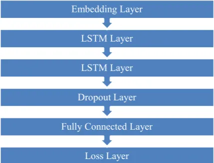
Recurrent layers are proved to be useful in han-dling variable length sequences (Tang et al., 2015). We use two series-connected long short-term memory (LSTM) cells to compute continu-ous representations of tweets with semantic composition.

Figure 3: Neural network structure.

3.3

We use dropout as the regularizer to prevent our network from overfitting (Srivastava, 2013). Our

2

http://radimrehurek.com/gensim/ Loss Layer Fully Connected Layer

dropout layer selects a half of the hidden units at random and sets their output to zero and thus prevents co-adaptation of the features.

3.4

The Sentiment140 dataset and all messages from SemEval Task4 competition since 2013 till 2016 were used (except sarcasm dataset) to pre-train neural network layers. Then we fine tuned them on the train subsets for extract subtask. We used Adam method for stochastic optimization of an objective function.

4

Experiment Methodology

This section describes our experimental setup for participation in the SemEval-2017 Task 4 called “Sentiment Analysis in Twitter”. Task 4 consists of five subtasks, but we only participated in top-ic-based message polarity quantification – sub-tasks D, E according to a two-point scale and five-point scale, respectively. Its dataset consists of Twitter messages (aka observations) divided into several topics. These subtasks are evaluated independently for different topics, and the final result is counted as an average of evaluation measure out of all the topics (Rosenthal et al., 2017).

For the quantification algorithm described in Section 2, we need to build a cost-sensitive clas-sifier in the function build_clf.

4.1

Last year we tried few cost-sensitive classifiers and finally chose a fast logistic regression classi-fier.

Since observation x in this dataset is a mes-sage written in a natural language, we first need to transform it to a vector representation X. Based on a study by (Gao and Sebastiani, 2015), we choose the following components of the fea-ture vector:

 TF-IDF for word n-grams with n varies from 1 to 4

 TF-IDF character n-grams where n varies from 3 to 5.

A feature vector is extracted with a Scikit_Learn tool3. We also perform data prepro-cessing. Several text patterns (e.g. links,

3

http://scikit-learn.org/stable/modules/generated/sklearn.feature_extractio n.text.TfidfVectorizer.html

cons, and numbers) were replaced with their sub-stitutes. For word n-grams we apply lemmatiza-tion using WordNetLemmatizer.

It is interesting to characterize messages using the SentiWordNet library. For each token xi in

document X we obtain its polarity value from the SentiWordNet. First, we recognize the part of speech using a speech tagger from the NLTK li-brary (Bird et al., 2009). Second, we get the SentiWordNet first polarity value for this token using the part of speech information.

The organizers provide a default split of the SemEval2016 data into training, development, development-time testing and testing datasets. The algorithms evaluation is performed using these subsets. The training, development and de-velopment-time testing subsets are used as a TRAIN set. The testing subset is used as a TEST set.

4.2

This year we try to apply neural network as a cost-sensitive classifier.

We remove punctuations from input text mes-sage. Then we split tweets into words and trans-form them into a sequence of word index with fixed length. All preprocessing is performed us-ing Keras4 library with Tensor Flow backend. We do not apply character sequences and lem-matization or stemming of words. As a TRAIN set, we use all datasets provided by organizers of topic-based message polarity challenge.

The chosen parameters of our network are as follows: the maximum input sequence length is set to 30, vocabulary size is 300000, the dimen-sionality of word embedding is 300, LSTM units hidden state vector size is 64, two LSTM layers and dropout of 50% while training. We use the dense layer with output dimension equals to one for subtask D and five for subtask E with sig-moid activation.

The metrics that we use to evaluate the classi-fier performance are described in (Rosenthal et al., 2017) and are not described here.

5

Experiment Results

The results of five point scale subtask are shown in Table 1. During the development period, we compare our system with last year one on the last year dataset. New system produced an EMD

4

measure of 0.347 while last year system was slightly better - 0.334. We explain this by the fact that dataset for network fine-tuning was rela-tively small last year. This year training dataset is three times bigger, that is why we decide to submit results from the new version of the algo-rithm.

EMD of our new system on the new dataset is 0.317 while the best system scored 0.245.

Settings EMD

Approach and dataset 2017 0.317 (5) Approach 2017, dataset 2016 0.347 Approach and dataset 2016 0.334 (4)

Table 1: Results of Task 4E.

The results of two-point scale subtask are shown in Table 2. Our algorithm shows KLD equals to 0.078 while the best system is 0.036.

Settings KLD RAE Approach and dataset 2017 0.078 (8) 1.528 (8) Approach and dataset 2016 0.084 (7) 0.767 (4)

Table 2: Results of Task 4D.

6

Conclusion and future work

The aim of this research was to try to solve sen-timent quantification task with deep learning ar-chitecture. We compared our deep learning ap-proach used this year with an apap-proach without deep learning used last year.

For tweet quantification on a five-point scale (Subtask E) and a two-point scale (Subtask D), we used the same iterative method proposed by (Xue and Weiss, 2009). As a classifier we used deep learning network which was retrained on the big corpus and fine tune on the small. These approaches showed the 5-th and the 8-th best places in the competition subtasks E and D re-spectively.

In our future work, we are planning to move in two directions. First, we plan to apply new deep architecture and pre-train it using more data. Se-cond, we want to explore the bias property of the CDE-Iterate quantification method.

Acknowledgments

The reported study was funded by RFBR under research Project No. 16-06-00184 A, the Aca-demic Fund Program at the National Research University Higher School of Economics (HSE) in 2017 (grant N17-05-0007) and by the Russian Academic Excellence Project "5-100".

References

Steven Bird, Ewan Klein, and Edward Loper. 2009.

Natural language processing with Python. O’Reilly Media, Inc.

Yee Seng Chan and Hwee Tou Ng. 2006. Estimating class priors in domain adaptation for word sense disambiguation. In Proceedings of the 21st Inter-national Conference on Computational Linguistics and the 44th annual meeting of the Association for Computational Linguistics, pages 89–96. Associa-tion for ComputaAssocia-tional Linguistics.

Andrea Esuli, Fabrizio Sebastiani, and Ahmed ABBASI. 2010. Sentiment quantification. IEEE in-telligent systems, 25(4):72–79.

George Forman. 2008. Quantifying counts and costs via classification. Data Mining and Knowledge Discovery, 17(2):164–206, June.

George Forman, Evan Kirshenbaum, and Jaap Suermondt. 2006. Pragmatic text mining: minimiz-ing human effort to quantify many issues in call logs. In Proceedings of the 12th ACM SIGKDD in-ternational conference on Knowledge discovery and data mining, pages 852–861. ACM.

Wei Gao and Fabrizio Sebastiani. 2015. Tweet Senti-ment: From Classification to Quantification. In

Proceedings of the 2015 IEEE/ACM International Conference on Advances in Social Networks Anal-ysis and Mining 2015, pages 97–104. ACM.

Alec Go, Richa Bhayani, and Lei Huang. 2009. Twit-ter sentiment classification using distant supervi-sion. CS224N Project Report, Stanford, 1(12).

A. Guerrero-Curieses, R. Alaiz-Rodriguez, and J. Cid-Sueiro. 2009. Cost-sensitive and modular land-cover classification based on posterior probability estimates. International Journal of Remote Sens-ing, 30(22):5877–5899.

David J. Hand and others. 2006. Classifier technology and the illusion of progress. Statistical science, 21(1):1–14.

Nikolay Karpov, Alexander Porshnev, and Kirill Rudakov. 2016. NRU-HSE at SemEval-2016 Task 4: Comparative Analysis of Two Iterative Methods Using Quantification Library. In Proceedings of the 10th International Workshop on Semantic Evaluation (SemEval-2016), pages 171–177, San Diego, California, June. Association for Computa-tional Linguistics.

Marco Saerens, Patrice Latinne, and Christine Decaestecker. 2002. Adjusting the outputs of a classifier to new a priori probabilities: a simple procedure. Neural computation, 14(1):21–41.

Lidia Sánchez, Víctor González, Enrique Alegre, and Rocío Alaiz. 2008. Classification and quantifica-tion based on image analysis for sperm samples with uncertain damaged/intact cell proportions. In

Image Analysis and Recognition, pages 827–836. Springer.

Nitish Srivastava. 2013. Improving neural networks with dropout. phdthesis, University of Toronto.

Duyu Tang, Bing Qin, and Ting Liu. 2015. Document Modeling with Gated Recurrent Neural Network for Sentiment Classification. In EMNLP, pages 1422–1432.

Lei Tang, Huiji Gao, and Huan Liu. 2010. Network quantification despite biased labels. In Proceedings of the Eighth Workshop on Mining and Learning with Graphs, pages 147–154. ACM.