Advancing the detection of steady-state visual
evoked potentials in brain-computer interfaces
Mohammad Abu-Alqumsan1 and Angelika Peer2
1 Chair of Automatic Control Engineering, Technical University of Munich (TUM), Munich, Germany
2 Bristol Robotics Laboratory, University of the West of England, Bristol, UK
E-mail: [email protected]
Abstract. Objective. Spatial filtering has proved to be a powerful pre-processing step in detection of steady-state visual evoked potentials and boosted typical detection rates both in offline analysis and online SSVEP-based brain-computer interface applications. State-of-the-art detection methods and the spatial filters used thereby share many common foundations as they all build upon the second order statistics of the acquired EEG data, that is, its spatial autocovariance and cross-covariance with what is assumed to be a pure SSVEP response. The present study aims at highlighting the similarities and differences between these methods. Approach. We consider the canonical correlation analysis (CCA) method as a basis for the theoretical and empirical (with real EEG data) analysis of the state-of-the-art detection methods and the spatial filters used thereby. We build upon the findings of this analysis and prior research and propose a new detection method (CVARS) that combines the power of the canonical variates and that of the autoregressive spectral analysis in estimating the signal and noise power levels. Main results. We found that the multivariate synchronization index (MSI) method and the maximum contrast combination (MCC) method are variations of the CCA method. All these three methods were found to provide relatively unreliable detections in low SNR regimes. CVARS and the minimum energy combination (MEC) methods were found to provide better estimates for different SNR levels. Significance. Our theoretical and empirical results demonstrate that the proposed CVARS method outperforms other state-of-the-art detection methods when used in an unsupervised fashion. Furthermore, when used in a supervised fashion, a linear classifier learned from a short training session is able to estimate the hidden user intention, including the idle state (when the user is not attending to any stimulus), rapidly, accurately and reliably.
Keywords: BCI, SSVEP, canonical correlation analysis, minimum energy combina-tion, multivariate synchronization index, maximum contrast combinacombina-tion, autoregres-sive spectral analysis
1. Introduction and Motivation
Steady-state visual evoked potentials (SSVEP) refer to the involuntary brain response to repetitive visual stimulation of the eye in humans and some non-human primates [1]. The measured scalp Electroencephalo-graphic (EEG) potentials are characterized in the fre-quency domain by constant amplitude and phase at the Fourier components of the stimulation frequency and its higher harmonics. SSVEPs can be observed when the driving frequency of the stimulus is in the range 4−100 Hz [2], below which the electrical excitations of the visual system is able to abate before the new stimuli are presented, and in this case, it is the tran-sient VEPs that can be observed [3]. Capilla et al. [4] showed that steady-state VEPs can be accurately pre-dicted from the linear summation of appropriately con-structed transient responses and concluded that both can be attributed to the same underlying neural mech-anism.
Due to several factors, SSVEP has been a core concept in non-invasive EEG-based brain-computer
interface (BCI) applications. Among these are its
robustness and relatively high signal-to-noise ratio (SNR), the high information transfer rate (ITR) it delivers and the short training time required, if any, before it can be used for online applications. Typically,
in SSVEP-based BCIs, different frequency-tagged
stimuli are displayed simultaneously with each stimulus given a predefined mapping to a system command. This mapping is also known to the user, who can control or communicate with the system, simply by attending to the stimulus corresponding to the command of interest. Relatively easy discrimination between the different frequencies is facilitated by the fact that selective attention to stimulus location modulates SSVEP [5].
Early investigated methods for SSVEP analysis and detection have relied mainly on Power Spectral Density Analysis (PSDA) with Fast Fourier Transform (FFT) applied on single-channel EEG data. Herewith, the temporal EEG signal is transformed into its Fourier representations where test statistics can be derived from obtained information about the power (or amplitude) [3, 6, 7, 8, 9], phase [10] or both [11], at all
considered driving frequencies. FFT-based methods
require relatively long data segments to give reasonable detection results since the frequency resolution (∆f) in the Fourier domain is determined by the reciprocal of
the temporal data length available (e.g. it is required to have a 4 s data segment to get a frequency resolution
of ∆f = 0.25 Hz). Known issues with FFT like the
grid effect (Fourier components cannot be computed for frequencies that are not an integral multiple of
∆f) and spectral leakage (energy spillover from one
frequency bin to adjacent ones due to rectangular windowing) highly affect the calculated amplitude and phase precision and should be accounted for by choosing suitable window functions and segment lengths [5, 12, 13]. In [14], authors argue that for an arbitrary steady-state recording, there might not be enough information to benefit from phase information in SSVEP detection.
Recently, there has been a great tendency to-wards different methods that rely on spatial filtering of multi-channel EEG data, which proved to be more efficient and stable than FFT-based methods. The ba-sic idea here is to find a spatial filter that transforms the original multi-channel EEG signals into single or multi-channels with desirable characteristics. Friman et al. [15] proposed the minimum energy combination (MEC) spatial filter, the first of its kind, which aims at minimizing the noise energy, with the noise defined as the orthogonal complement to the projection of the EEG signals onto the subspace spanned by the pure SSVEP vectors. Alternatively, the canonical correla-tion analysis (CCA) aims at finding a pair of spatial lin-ear combinations for both, the EEG signals and the as-sumed pure SSVEP responses, which jointly maximize the correlation between the resulting canonical vari-ates [16]. The maximum contrast combination (MCC) filter maximizes the signal-to-noise ratio, defined with
the generalized Rayleigh quotient [15, 17]. Finally,
the multivariate synchronization index (MSI), through spatial whitening, extracts a single metric that reflects the synchronization level between the EEG signals and assumed pure SSVEPs [18].
The main contribution of this work is that we show the similarity of the spatial filters and the scoring functions used by the standard unsupervised CCA, MSI and MCC approaches to SSVEP detection, where we conclude also that their detection accuracies should not differ significantly. We show additionally that these methods, in low signal-to-noise ratio (SNR) regimes, fail to provide a reliable detection as they ignore the noise power in the spontaneous EEG that overlaps the stimulation frequencies.
like autoregressive methods, are able to provide an estimate for the noise power levels after removing the total energy of the driving frequencies from
the spatially filtered signals. This was shown to
provide reliable test statistics for SNR that can be
used for SSVEP detection [15, 19]. Based on the
theoretical analysis of these state-of-the-art methods,
we propose a new method, namely the canonical
variates with autoregressive spectral analysis(CVARS) that estimates the signal and noise power levels from the canonical variates which leads to slight improvement in correct detection rates. This method, when used in a supervised fashion, results in a rapid, accurate and reliable SSVEP detection regardless of the level of SNR as shown from the experimental results with real EEG data. We additionally show the conditions on which the MEC-based detection provides similar results to the CVARS method.
2. Preliminaries
2.1. Notation
We use bold uppercase letters (e.g. Z) to denote two-dimensional matrices and bold lowercase letters (e.g.
z) to denote column vectors, and conversely zT for
row vectors. The Frobenius norm of the matrix Z is
denoted bykZkF.
A p-variate random variable is denoted by an
uppercase letter, where it refers to a vector ofprandom variables, e.g. Z = [Z1, Z2, . . . Zp]. Realizations of
Z are denoted the same way as vectors (e.g. z). A
sequence of n p-dimensional vectors is concatenated
in the sample data matrixZ= [z1,z2, . . .zn]T, where
Z ∈ Rn×p. The expectation of a random variable
Z is denoted by E[z] and E[z], for one and
multi-dimensional variables, respectively. For an arbitrary
matrix Z ∈ Rn×p, σ(Z) = (σ
1, σ2, . . . σmin(n,p))
denotes the singular values of Z, where σ1 ≥ σ2 ≥
. . . σmin(n,p) ≥ 0. For arbitrary square matrix Z ∈
Rn×n, λ(Z) = (λ
1, λ2, . . . λn) denotes the eigenvalues
ofZwithλ1≥λ2≥. . . λn. The dominant eigenvalue is
denoted by λ1(Z) or λmax(Z). An arbitrary diagonal
matrix D ∈ Rn×n can be defined with its diagonal
elements as diag(d1, . . . , dn).
The autocovariance matrix of p-variate random
variableX is denoted byCxxand the cross-covariance
matrix between two random vectors X and Y is
denoted by Cxy. Often in practice, the true value of such covariances remains unknown, and therefore they are replaced by the sample auto and cross-covariance
matrices Qxx and Qxy, computed from the centered
sample matrices with Qxx = N1XTX and Qxy =
1 NX
TY, whereN is the number of available samples
in X and Y. Unless explicitly stated otherwise, all
sample matrices encountered here will be centered or
made centered by subtracting the sample mean from all observations.
2.2. Background
We assume that after the retina is excited by flickering light, and after the transient VEPs vanish [20], pure SSVEP responses appear as multiple phase-shifted sinusoidal waves whose frequencies are integer multiple (up toNh) of the driving frequency. The assumed pure waves propagate to the scalp where EEG signals are measured. Due to volume conduction of the head, a linear combination of these source signals corrupted with noise will be observed at each measurement location, i.e. electrode. The additive noise might have encephalic or non-encephalic sources, and is generally non-stationary. However, for short EEG segments, it is often assumed to be stationary in the wide sense [21]. No statistical knowledge about the noise is additionally assumed here. Formally, we state that in response to flickering light with driving frequency f, the values recorded over time at each electrode ican be written as
yi(t) = Nh X
h=1
ai,hsin(2πhf t+φi,h) +ψi(t), (1)
where i ∈ {1, . . . , Ny} and Ny is the total number
of recording electrodes. The terms ai,h and φi,h ∈
]−2π,0] respectively denote the harmonic-specific
amplitude and phase lag at electrode i. The additive
noise contributing toyi(t) is denoted byψi(t). For the
digitized EEG with sampling rate of Fs (in Hz), (1)
becomes
yi[k] = Nh X
h=1
ai,hxi,h[k] +ψi[k], where (2)
xi,h[k] = sin(2πhf k
Fs
+φi,h)
= sin(2πhf k
Fs
) cos(φi,h) + cos(2πhf k
Fs
) sin(φi,h).
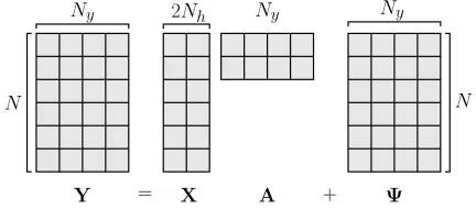
With conformable transformation of the ampli-tude values ai,h, the above notation can be rewritten for a collection of N samples from all Ny electrodes (see figure 1) in matrix form as
Y=XA+Ψ. (3)
Here,Y=
y1 y2 · · · yNy,Ψ∈RN×Ny and
the propagation (or mixing) matrix A ∈ R2Nh×Ny.
The source model matrixX∈RN×2Nh is defined now as
X=X1 X2 · · · Xh · · · XNh
, (4)
where Xh = [sin(2πhf k0) cos(2πhf k0)]∈RN×2, and
k0 =Fs1,Fs2, . . . ,FsN.
In absence of any statistical knowledge about the
Ny Ny Ny
N N
2Nh
[image:4.612.69.285.61.156.2]Y = X A + Ψ
Figure 1: Matrix representation of the EEG model
containing SSVEPs
the acquired EEG data by ALS = (XTX)−1XTY
which minimizes the total least squares error, i.e.
kY−XAk2
F. Equivalently, the LS estimate of ALS
can be written asALS=Q−xx1Qxy, whereQxxandQxy respectively denote the sample spatial autocovariance matrix of the pure SSVEP response and the sample cross-covariance between the acquired EEG data and
the assumed source model, both are estimated fromN
observations. Despite the fact that the source signals are defined deterministically, they can be modeled as stochastic with empirical means computed on segments of lengthN, which can be approximated with the
zero-vector 0 for large N. Due to the orthogonality of
the basis vectors in X, the sample covariance matrix
Qxx, for centered and normalized X, can also be
approximated for relatively large N with INx, where
Nx = 2Nh. In this formulation, the number of
harmonics in the SSVEP response, i.e. Nh, is not a
random variable but rather an unknown deterministic value.
Where it is necessary, in order to avoid ambiguity when we refer to the source model for the different driving frequencies, the subscript f will be added to matrixXf to indicate the source model of the driving frequency under consideration.
2.3. Stimulus identification during SSVEP-based interaction
During concurrent repetitive visual stimulation, an SSVEP detector aims at finding the stimulus, at which the user is attending, based on multi-channel EEG data segmentY∈RN×Ny, obtained online from continuous scalp EEG data by means of buffering (with buffer
length N and buffer overlap O where 0 ≤ O <
N). Based on the requirements of the application at
hand, the buffer length and the interaction temporal
resolution (T) are determined. T is defined as the
shortest time (in samples) between two consecutive
commands. The overlap can be computed from O =
max(0, N−T).
The problem of stimulus identification from EEG
data thus can be formulated as having M
spatially-Buffered EEG Data Y∈RN×Ny
Scoring Function (e.g. CCA-based, MSI-based, MEC-based,. . .) Source
Models Xf∈RN×Nx
Continuous EEG Data s
Buffer LengthN
[image:4.612.318.532.62.157.2]O T
Figure 2: Schematic of a general SSVEP detector from continuous EEG data. Different scoring functions can be used to provide the score vectors∈RM+1, whereby
a decision about the user intention can be made every
T samples.
distributed flickering lights, driven by different
frequen-ciesf1, f2, . . . , fM, and a mapping function ˆgis sought,
where ˆg :RN×Ny 7→ {f
0, f1, . . . , fM}, and f0 denotes
the idle state, i.e. when the user does not attend to any of the stimuli. Often, ˆg(Y) is defined as the argument which maximizes a score function or a test statistic s. SSVEP detection can be formally written as
ˆ
f = ˆg(Y) = argmax
fl∈{f0,f1,...,fM}
s(Y,Xfl). (5)
We denote byg(Y) the ground truth frequency of the
stimulus, to which the user attends while Y is being
acquired. The score s(Y,Xf0) is considered here as
to test whether or not a given response is statistically significant and not due to noise fluctuations and background EEG. More often than not, it is defined as a constant threshold which is either computed from the EEG data segments themselves or a priori computed from training data. For completeness, let
s ∈ R(M+1)×1 denote the vector containing the score
value for all frequencies plus the idle state.
Figure 2 depicts the schematic of SSVEP detection in continuous EEG data. Available scoring functions used in (5) will be discussed in section 3.
2.4. Evaluation
The different detection methods, which will be
discussed later, are compared with regard to their average accuracy ( ¯PD), which is typically computed from labeled EEG segments as the ratio of the correctly classified segments to the total number of available segments. Average misclassification error can be easily computed withEm= 1−P¯D.
2.5. Challenges in SSVEP-based interaction
state. Obviously, such interaction is asynchronous and completely paced with the user actions. However, and regardless of the SSVEP detection method used, recog-nition of these asynchronous spatial attention shifts does not happen usually on the spot due to inher-ent limiting factors of the buffering stage. The shorter the buffer size (small N and T), the faster is the re-sponse of the system. With larger buffer sizes, however, the temporal random fluctuations in the score func-tion s(Y,Xf) are made less severe as the noise (the assumed source of variability in the evoked potentials) attenuates typically in proportion to the square root of the number of time averages done on the data. On the other hand, larger buffer sizes introduce delays into the system and reduce the achievable bit rate. Con-sequently, finding a trade-off between interaction ac-curacy and speed is of high importance for practical systems.
3. SSVEP detection methods
In the next subsections, we will provide the theoretical background for the spatial filtering methods used in state-of-the-art SSVEP detection and show in which ways they differ and how the spatial filters obtained are related to each other. Additionally, we propose a new detection method that performs superiorly in different SNR regimes as it combines CCA spatial filtering and autoregressive spectral analysis to estimate the signal and noise levels at all possible driving frequencies.
3.1. Canonical correlation Analysis (CCA)
Lin et al. [16] used canonical correlation analysis (CCA) to recognize the narrow-band driving frequency of SSVEPs from EEG data. The CCA-based method was found to outperform the FFT-based spectrum estimation method in terms of classification accuracy. This result has been repeatedly reported in [8, 22]. The superior performance can be attributed to the ability of CCA to reveal spatial coherence in data contaminated by either white Gaussian noise or colored noise fields, should the data have high SNR [23].
CCA [24] does that by finding the maximally correlated pairs among all possible linear combinations
of two zero-mean multivariate random variablesXand
Y, wherex∈RNx×1 andy∈RNy×1. Without loss of
generality, we assume in the following thatNx≤Ny. Formally, we look for the canonical weight vectors
wx and wy where x = wxTx and y = wTyy, such
that the correlation coefficient between the canonical
variatesxandy,ρ1(x, y) is maximized. By definition,
ρ1(x, y) =
E[xy]
p
(E[x2]E[y2])
= E[w
T
xxyTwy] q
E[wT
xxxTwx]E[wTyyyTwy]
= w
T
xE[xyT]wy q
wT
xE[xxT]wxwTyE[yyT]wy
= w
T xCxywy q
wT
xCxxwxwTyCyywy
. (6)
Since scaling ofwxandwy doesn’t affect the objective function, the search space is limited by constraining the variance of the variatesxandy to be 1 [25]. This leads to the new optimization problem
wx,wy= argmax
wx,wy
wTxCxywy
subject to wTxCxxwx=wTyCyywy = 1
By introducing Lagrange multipliers, one can easily obtain the following generalized eigenvalue problems
CxyC−yy1Cyxwx=ρ21Cxxwx (7) CyxC−xx1Cxywy=ρ21Cyywy. (8)
Due to the fact that Cxx and Cyy denote
covariance matrices, which are symmetric positive semi-definite, (7) and (8) can be rearranged into two standard symmetric eigenvalue problems,
TTTw0x=ρ21w0x, (9)
TTTw0y=ρ21w0y, (10)
where T = C−xx1/2CxyC
−1/2
yy , w0x = C 1/2
xxwx and similarlyw0y=C1yy/2wy. The matrixTis referred to as thecoherence matrix and denotes the cross-covariance between the whitened vectors C−xx1/2x and C−
1/2 yy y. This yields thatρ1(x, y) =σmax(T) =
p
λmax(TTT).
The matrix productTTT is often referred to assquared
coherence matrix [26]. Other uncorrelated canonical
variates can be found using the remaining eigenvectors and eigenvalues [25].
For later use, we define the decompositionTTT= W0
yP 2W0T
y , where Wy0 ∈ RNy×Nx and P has all
the canonical correlations on its diagonal, i.e. P =
diag(ρ1, ρ2, . . . , ρNx) = diag( p
λ(TTT)). Similarly, TTT =W0
xP 2W0T
x , whereW0x∈RNx×Nx.
The score function in (5) can thus be defined for the standard CCA method asscca=ρ1. Alternatively,
other score functions can be derived as an arbitrary function of (ρ1, . . . , ρNx), in the formsfcca=f(σ(T)).
Xf4
Xf2
Xf3
Xf1
Y
{θ2
i}
{θ4
i}
{θ3
i}
{θ1
[image:6.612.83.283.64.231.2]i}
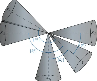
Figure 3: Principal angles between the subspaces
spanned by the different source models and the
acquired EEG data. Each is a subspace in RN and
is represented by a convex cone. Note also that the column spaces of the differentXflmay intersect if they share, at least, one basis vector, as it is the case with
Xf1 andXf3, wheref1= 15 andf3= 10, andNh= 3.
Given enough samples forY, i.e. N Ny, thenQyy
will be full rank and invertible.
Equivalently, the canonical correlations [27] can be found by first applying the QR decomposition
of Y = QyRy and X = QxRx, to obtain the
orthonormal matricesQxandQyand the full rankRx andRymatrices. The second step involves the singular value decomposition of QTxQy asUPVT, where U=
1
√
NRxWx andV= 1
√
NRyWy
This formulation is computationally more effi-cient and provides more insights on the geometric in-terpretation of CCA. Hereby, the canonical correla-tions correspond to the cosine of the principal an-gles between the two subspaces spanned by the col-umn spaces of Qx and Qy or formally, σ(QTxQy) =
cos(θ1), . . . ,cos(θmin(Ny,Nx))
. Geometrically, the
maximum canonical correlation is the cosine of the smallest angle possible between any two vectors in the subspaces spanned byQxandQy. Figure 3 illustrates this relation.
3.2. Multivariate Synchronization Index (MSI)
More recently, Zhang et al. [18] introduced the
multivariate synchronization index (MSI) for online SSVEP detection, where the synchronization level between the source model and the acquired EEG is
measured based on the S-estimator [28]. The joint
covariance matrix CX,Y which includes the auto and
cross-covariance matrices of Xand Y can be written
in block form as
CX,Y =
Cxx Cxy Cyx Cyy
. (11)
The transformUthat orthogonalizes the diagonal
block matrices, i.e. whitens the original data matrices
XandY, was applied such thatR=UCX,YUT and
U=
"
C−xx1/2 0 0 C−yy1/2
#
,R=
INx T TT INy
, (12)
where T = C−xx1/2CxyC
−1/2
yy is the coherence matrix
already encountered. Let P = 2Nh +Ny, λ(R) =
(λ1, . . . , λP), and the normalized eigenvalues to be
defined as λ0i = λiP. The synchronization index then can be obtained from the entropy-like quantity
smsi= 1 + PP
i=1λ0ilog(λ0i)
log(P) . (13)
The MSI-based score is tightly related to scca, as
the eigenvalues of R are nothing more than a simple
transformation of the canonical correlations, such that λi = 1 +ρi,∀i ∈ {1, . . . , Nx}, λi = 1−ρi,∀i ∈
{Nx+1, . . . ,2Nx}andλi= 1, otherwise (see Appendix A). This renders smsi as a mere nonlinear function of
all canonical correlations, and as special case of the sfcca. Additionally, the filtering step (i.e. whitening)
involved is similar to that in the CCA method.
3.3. Minimum Energy Combination (MEC)
Friman et al. [15] proposed to apply the spatial filter
WMEC ∈ RNy×Ns, which minimizes the noise energy
in S = YWMEC ∈ RN×Ns, where N
s ≤ Ny. The noise here is defined as the difference between the original EEG signal and its best LS approximation in the subspace spanned by the SSVEP sinusoids. The noise is thus estimated as
˜
Ψ=Y−XALS=Y−XQ−xx1Qxy. (14) Note thatscca( ˜Ψ,X) = 0. The sample noise covariance
matrix can be written as Qψψ =Qyy −QyxQ−xx1Qxy with the eigendecomposition QψDψQTψ. The spatial
filter WMEC is then obtained by concatenating the
last Ns vectors in Qψ which correspond to the
least proportion of energy in ˜Ψ, e.g. correspond
to the eigenvalues whose sum does not exceed Tr(Qψψ)/10 [15].
A test statistic can be derived from the filtered signals, to which we will refer as smec(Y,X) and is
obtained with [15]
s(Y,X) = 1
NsNh
Ns X
l=1 Nh X
k=1
ˆ
Pkl
ˆ
σ2
kl
, (15)
where ˆPkl =kXTkslk2 estimates the signal power and ˆ
σkl provides an estimate to the noise power at the k-th harmonic in k-the lth spatially filtered signal. σˆ
is obtained by fitting a p-order autoregressive AR(p) model, with parameters{αˆl1, . . . ,αˆlp,σˆ2l} to the data of each column (l) in the matrix
˜
S= S−X(XTX)−1XTS= ˜ΨW
MEC ∈ RN×Ns [15],
wherel∈ {1, . . . Ns}. It can be computed as
ˆ
σkl2 = πNσˆ
2 l/4
|1 +Pp
m=1αˆlmexp(−j2πmkf /Fs)|2
,
wherej=√−1,Fsis the sampling frequency andf is the stimulation frequency.
The discrimination power of the statistic in (15) stems from its ability to incorporate the noise power
estimate at the frequencies under consideration. So
far, the score functions in CCA and MSI reflected the signal power only. Furthermore, we can write the noise covariance matrix as
Cψψ =Cyy−CyxC−xx1Cxy =Cyy INy−C
−1
yyCyxC−xx1Cxy =Cyy
INy−C
−1/2 yy T
TTC1/2 yy
=Cyy
INy−C−yy1/2W
0
yP 2
W0yTC1yy/2
=Cyy
C−yy1/2W0y INy−P2
W0yTC1yy/2
=C1yy/2W0y INy−P2
W0yTC1yy/2 (16) =CyyWy INy−P2
WTyCyy. (17)
Multiplying both sides withWT
y from the left andWy from the right, yields the following relation
WTyCψψWy=INy−P2. (18)
Therefore it is possible to diagonalize the noise covariance matrix with the canonical weights matrix
Wy, which is generally not orthogonal, as by definition WT
yCyyWy = INx. Recall that the diagonalization
of Cψψ = QψDψQTψ in the original paper of the
MEC method was done with eigendecomposition [15]. Should the EEG data be spatially white or
pre-whitened, i.e. Cyy = INy before running the MEC
procedure, and Ns is fixed to 2Nh, then Wy =
W0y = Qψ, This result provides another intuitive
insight on the MEC filtering. When the original
EEG signals is pre-whitened, MEC maximizes the canonical correlation coefficients while minimzing the noise energy since the smallest diagonal elements in
Dψand INy −P2
correspond to the largest canonical correlations.
3.4. Maximum Contrast Combination (MCC)
The goal of the maximum contrast combination (MCC) method is to find the linear spatial filter that maximizes the generalized Rayleigh quotient[15,
17]. Formally, we are after w which maximizes
λ = w
TCyyw
wTCψψw subject to kwk2 = 1. The true
covariance matrices are not known and thus they are substituted with their sample estimates. The sample
noise covariance matrix Qψψ can be found the same
way as in section 3.3. With the help of Lagrangian
multipliers, one can show thatλattains its maximum
with the dominant eigenvector of the matrixC−ψψ1Cyy, which can be rewritten with the result in (16) as
Cψψ−1Cyy =Cyy−1/2W0y INy −P2 −1
Wy0TC 1/2 yy . (19)
Thus, λi(C−ψψ1Cyy) = 1/(1−ρ2i) = fmcc(ρi) , ∀i ∈
{1, . . . ,min(Nx, Ny)}, and consequentially, λmax =
1/(1 −ρ2max). The spatial filter w which attains
the maximum quotient can be found by normalizing the columns C−yy1/2W0y = Wy with respect to the Euclidean norm, and picking the one corresponding to
ρmax. This proves that MCC and the CCA methods
have exactly the same discrimination power since the functionfmcc(ρ1) is monotonically increasing inρ1.
3.5. Canonical variates with autoregressive spectral estimation of noise (CVARS)
As stated earlier, the standard CCA method is able to reveal spatial coherence in high SNR regimes.
When SNR 1, however, the canonical coefficients
mainly reflect the correlation between the noise and the assumed source signals, which often leads to erroneous detection as the separate contribution of the signal and the noise to the total values ofρicannot be determined. Therefore, we propose to estimate the noise at each frequency for each signal after spatial filtering with parametric spectral density estimation. That is, the noise power is estimated by fitting an autoregressive model to canonical variates after cleaning them from all energy at the SSVEP driving
frequencies and their higher harmonics. The test
statistic scvars is computed exactly as in (15) with
the AR(p) models fitted on ˜S=S−X(XTX)−1XTS,
where S=YWy andWy ∈RNy×Nx is the canonical
weighting matrix. Additionally, we observe that
XTS=NW
xPand therefore ˆPkl =N ρ2l(w 2 kl,1+w
2 kl,2),
where wkl,1 and wkl,2 denote the respective weight of
the sine and cosine signals of thekth harmonic in the lthcanonical variate.
3.6. Discussion
In the light of the previous analysis and findings, it is obvious that the scores of the CCA, MCC and MSI methods correspond to different functions of the canonical correlations (ρi), and their scores can all be considered special cases of sfcca. Common to all of
necessary to do so to obtain the scoring functionsscca
andsmcc, these methods additionally involve applying
the transform C−yy1/2 to the left singular vectors of the coherence matrix in order to obtain the optimal
spatial filter. The spatial filtering of the MEC and
CVARS methods is accomplished with the eigenvectors of the noise covariance matrix and the canonical weighting matrixWy, respectively. Additionally, both involve spectral analysis of AR(p) models fitted on the spatially filtered data cleaned from the energy at the driving frequencies of the SSVEP. The rationale behind using (3.3) in [15, 19] is that the temporally colored noise in each column ˜sl in the matrix ˜S, can be modeled as discrete-time autoregressive random process of orderp, such thatPp
k=0αks[n˜ −k] =u[n],
where u[n] is white Gaussian noise of power σ2 and
α0= 1. As a result, this modeling allows to whiten the
temporally colored noise, and produce an unbiased (or with small bias [19]) estimate for the noise power at each stimulation frequency and its higher harmonics. The CVARS method, therefore, involves whitening the data, both spatially and temporally, before it can provide the scoring function scvars. If the data
is spatially pre-whitened before applying the MEC method, then results will be very similar to those of
the CVARS method, but not exactly the same as Ns
used to computesmec is governed by a fraction of the
total energy in the noise signal and in case of CVARS, Ns= 2Nhis fixed.
4. Material and methods
In order to compare the different detection methods, several experiments with volunteer subjects were conducted.
4.1. Subjects
A total of 10 healthy adults (1 female) aged 29.3±
5.5 (range 22 − 39) with normal or
corrected-to-normal vision served as paid volunteer subjects in this study. During the experiments, the participants were seated 0.65 m away from an LCD monitor on a comfortable armchair in a slightly dimmed room. All participants gave their written informed consent. Participants were additionally asked to fill in pre-and post-questionnaires, that were meant to collect data about the level of tiredness before and after the experiment in addition to some demographical data.
Scalp EEG signals were recorded from 16
electrodes positioned according to the international extended 10/20 electrode system over the parieto-occipital scalp areas at P3, Pz, P4, PO9, PO7, PO3, POz, PO4, PO8, PO10, O9, O1,Oz, O2, O10 and
Iz. Electrodes were referenced to the right earlobe
and the ground electrode was positioned at FPz. The
Forward
TurnL TurnR
[image:8.612.324.527.58.187.2]Stop
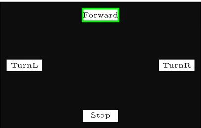
Figure 4: Stimulus presentation. In synchronization with the display refresh rate, four white rectangles were flickered on and off against a black screen at rates of 15 Hz (Forward), 12 Hz (TurnL), 10 Hz (TurnR)
and 8.57 Hz (Stop). The labeling of the different
rectangles serves robotic control applications. The size proportions between the flicker and the display are preserved in the figure.
signals were acquired with sampling rate of 512 Hz using g.USBamp acquisition system (g.tec medical engineering GmbH, Schiedlberg, Austria) and band-pass filtered at 0.5−60 Hz. The power line interference
at 50 Hz was removed with a 4th order butterworth
notch-filter with 48−52 Hz stop band. All electrodes were filled with highly conductive gel in order to reduce impedance.
This study is part of a larger project, which is approved by the Ethics Committee of the Faculty of Medicine of the Technical University of Munich (TUM).
4.2. Experimental paradigm
A 2200 liquid-crystal display (LCD) monitor‡ with
60 Hz refresh rate and 1280 × 1024 resolution
was used to view the stimuli which consisted
of four spatially distributed flickering rectangles presented simultaneously to participants. The driving
0 3.5 13.5 17 27 30.5 40.5 44 54 57.5 Off
On
15Hz 12Hz 10Hz 8.57Hz
time (s)
Stim
ulation
[image:9.612.79.286.59.150.2]10 sec 3.5 sec
Figure 5: Trigger timing for one complete stimulation
sequence. When stimulation is on, all flickering
stimuli are presented concurrently. Each stimulus
is highlighted for 10 seconds as shown with the stimulation train signal.
frequencies of the stimuli were chosen as integer divisors of the display refresh rate, namely 15, 12, 10 and 8.57 Hz. The chosen andfixed driving frequencies are known to evoke moderate to high SSVEP’s amplitude strength [29]. The spatial distribution of the stimuli is shown in figure 4. The EEG acquisition and visual stimulation were running on two different computers, and synchronized with the screen overlay control interface (SOCI) [30, 31].
Two recording sessions were performed, each started with a blank screen for around 15 seconds followed by the presentation of the flickering stimuli. During stimulation, participants were instructed to overtly sustain the spatial attention on the cued stimulus. Stimuli were highlighted in turn with a green rectangle as shown in figure 4 for 10 seconds followed by a rest period of 3.5 seconds, in which the screen went blank. The stimuli were cued in the descending order of their driving frequencies (i.e. the sequence will be top, left, right and bottom according to the stimuli constellation shown in figure 4). Detailed timing of one complete sequence is shown in figure 5. Each recording session consisted of five such full sequences.
5. Experimental Results
The accuracy for each of the different detection methods is highly influenced by the choice of the
key system parameters, e.g N, T, Nh and Fs. In
the following, we will firstly highlight the effect of each of these parameters individually on unsupervised CCA detection accuracy. We chose the CCA method here as the other scoring functions can be obtained from the canonical coefficients, canonical variates and the canonical weights, and thus it can serve as an indicator of the information gain/loss that
accompanies parameter change. By fixing these
parameters in the light of the empirical evaluation of CCA, the unsupervised detection accuracy of the CVARS is then compared to the state-of-the-art
Buffer Size [s]
A
v
e
ra
g
e
m
is
c
la
ss
i
fi
c
a
ti
o
n
e
rr
o
r
(
Em
)
0.1
0.2
0.3
0.4
0.5
0.6
0.7
0.5 1 1.5 2 2.5 3 3.5 4 4.5 5
S1 S2
S3 S4
S5 S6
S7 S8
S9 S10
mean
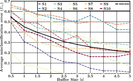
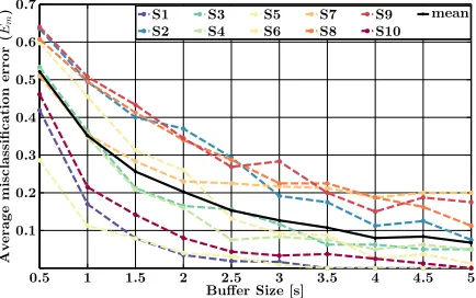
Figure 6: Average misclassification error for CCA
computed as Em = 1−P¯D for varying buffer length,
Nh= 1.
methods.
5.1. CCA results with varying key system parameters
Labeled non-overlapping EEG data segments (i.e. O=
0) are extracted from the two available recording
sessions per subject. The segment size was varied
between 0.5 −5 seconds with steps of 0.5 seconds,
respectively yielding 200, 100, 60,50,40,30,20,20,20 and
20 segments, per stimulation frequency. Segments
which were obtained during the idle state were not included in the evaluation since we consider unsupervised CCA at this stage.
Figure 6 shows the average misclassification error (Em) for all subjects as a function of the buffer size,
when the CCA method was used with Nh = 1 and
Fs = 512 Hz. With larger buffer sizes, one can
observe that misclassification errors for all subjects get suppressed due to enhanced SNR and more accurate estimates ofQyy and Qxy.
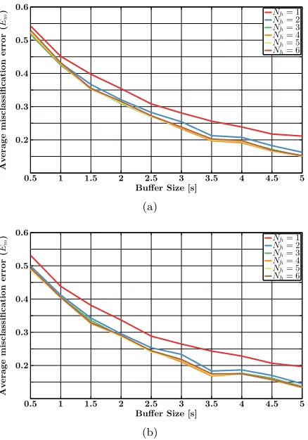
Figure 7(a) shows the average misclassification error of the CCA method (averaged over all subjects) for different number of harmonicsNhthat ranges from 1 to 6 as a function of buffer length. For Nh > 3, no further improvement is observed, which cannot be explained by the fact that EEG data itself was lowpass-filtered with a cutoff frequency 60 Hz since the fourth harmonic of the maximum stimulation frequency is not rejected thereby. However, the fourth harmonic
of the driving frequency f2 = 12 Hz, lies within
the stop band of the notch filter. In order to fully
isolate the influence of the notch filter, we reevaluated the average misclassification error of the unsupervised
CCA method (excludingf2 from the analysis). Again,
[image:9.612.311.531.61.196.2]Buffer Size [s] A v e ra g e m is c la ss ifi c a ti o n e rr o r ( Em )
0.2
0.3
0.4
0.5
0.6
0.5 1 1.5 2 2.5 3 3.5 4 4.5 5
Nh= 1 Nh= 2 Nh= 3 Nh= 4 Nh= 5 Nh= 6
(a)
Buffer Size [s]
A v e ra g e m is c la ss i fi c a ti o n e rr o r ( Em )
0.2
0.3
0.4
0.5
0.6
0.5 1 1.5 2 2.5 3 3.5 4 4.5 5
Nh= 1 Nh= 2 Nh= 3 Nh= 4 Nh= 5 Nh= 6
[image:10.612.61.280.58.371.2](b)
Figure 7: Average misclassification error for CCA
computed with different number of harmonics. For
Nh > 3, no further improvement in accuracy is
observed. Evaluation is based on (a) all stimulation frequencies (b) and execludingf2= 12 Hz.
As has been mentioned earlier, one can derive arbitrary scoring functions sfcca from the canonical
correlationsρi. Figure 8 shows the results for sfcca = Pk
1ρi, while fixing Nh = 3, and k ∈ {1,2, . . .2Nh}.
The performance degradation of sfcca for k > 1
suggests that the fluctuations in ρi,∀i > 1 over time cannot be used in winner takes all (WTA) assignment asρ1 for SSVEP detection.
The effect of changing the sampling rate is shown in figure 9. Downsampling with a factor of 2 or 4, which respectively resembles sampling frequency of 256 and 128 Hz leads to accuracies that are comparable with
the full data segments (with Fs = 512). Estimation
of covariance matrices Qyy andQxy is not, therefore, significantly affected by downsampling. This behavior suggests that adjacent samples inYare correlated (and
they are) and that allowing for ∆t between samples
that is larger than the expected maximum correlation
lag would not affect the obtained results. Going
to downsampling factor of 8 (Fs = 64) deteriorates
the performance significantly, as this would introduce
Buffer Size [s]
A v e ra g e m is c la ss ifi c a ti o n e rr o r ( Em )
0.2
0.3
0.4
0.5
0.6
0.5 1 1.5 2 2.5 3 3.5 4 4.5 5
k= 1
k= 2
k= 3
k= 4
k= 5
[image:10.612.312.529.60.195.2]k= 6
Figure 8: Average misclassification error for CCA
averaged over all frequencies and subjects computed for different scoring function ofρi andi∈ {1, . . . , Nx}.
aliasing and loss of information of the higher harmonics (with frequencies larger than Fs/2). Throughout the remaining of this work, we useFs= 512 Hz. Sampling ratesFs∈ {256,128} are expected to produce similar results in terms of the reported scores and the reported misclassification rates.
Buffer Size [s]
A v e ra g e m is c la ss i fi c a ti o n e rr o r ( Em )
0.1
0.2
0.3
0.4
0.5
0.6
0.7
0.5 1 1.5 2 2.5 3 3.5 4 4.5 5
d= 1 d= 2 d= 4 d= 8
Figure 9: Average misclassification error for CCA
averaged over all frequencies and subjects for different downsampling factors. Hardly any difference is noticed
for d ∈ {1,2,4}. When the downsampling factor
is 8 (the dotted purple line), significant reduction in accuracy is observed.
The estimates of the detection accuracies obtained so far using the non-overlapping data segments can be a bit misleading as classification is performed only
on homogeneous EEG data segments, during which
subjects attended to one single driving frequency. However, during online usage, EEG data collected in one segment can reflect two or more different states of user attention (e.g. user shifts his attention from one stimulus to another or from the idle state to
one of the active states within the segment). This
behavior becomes more probable with larger buffer
[image:10.612.311.529.342.482.2]data segments (i.e. T = 1 sample) were continuously extracted from the data and used to plot the CCA score evolution of the different stimulation frequencies over time. The resulting segments thus contain both
homogeneous and heterogeneous data. In order to
additionally provide more insights about the inter-subject variability in figure 6, the score evolution
will be shown for the subjects S5 and S2, whose
CCA results were the best and the worst, respectively. CCA score evolution during the first full sequence (after viewing all stimulation frequencies once) for (N, T) = (1024,1) samples is shown in the upper row of figure 13. These plots show, to some extent, that during stimulation withf, the scores(Y,Xf) increases over time and surpasses the scores of the other frequencies. Additionally, among the used stimulation frequencies, one can observe for each subject, that a specific frequency is somewhat dominant throughout
the whole sequence (12 Hz for S5 and 10 Hz for
S2), and to this specific frequency most of the faulty detections and false alarms can be attributed. While high scores for the dominant frequency (most likely due to interference from the alpha brain band waves, within which a peak can be observed in most subjects’ EEG[32]) starts to appear during the idle state, they get suppressed (though not always) when subjects shift their visual attention to flickering light. Furthermore, one can categorize the SSVEPs of the two subjects into high and low SNR with respect to the obtained CCA score values, whereS2 is the one with the low SNR.
5.2. Distribution of canonical correlations
In the following, we will refer to the canonical correlation values obtained when users attended to
a specific stimulus with frequency f as the target
canonical correlations (or target scores) for that frequency. Nontarget scores of a stimulation frequency f, on the other hand, refer to the values obtained when the user attended to other or no stimuli. By fixing
Nh= 3 and (N, T) = (1024,1) samples, we computed
the target and nontarget correlation coefficients for all stimulation frequencies in all recording sessions for all subjects. We assigned a data segment to a frequency f, if the most recent sample in the buffer was obtained when the corresponding stimulus was then cued for viewing.
From the histogram of all these values, we estimated the distribution of all target and nontarget canonical correlations which are shown in figure 10. These plots show that the difference between the distributions of the target and nontarget canonical
correlations ρi is most pronounced for ρ1. Most
importantly, we could see that the typical means (for all canonical correlations) per stimulation frequency differ significantly, in a way that reflects the general
Stimulation Frequency
C
a
n
o
n
ic
a
l
C
o
r
r
e
la
ti
o
n
V
a
lu
e
0.1 0.2 0.3 0.4 0.5 0.6 0.7 0.8
8 9 10 11 12 13 14 15 16
ρ1
ρ2
ρ3
ρ4
ρ5
[image:11.612.311.529.62.198.2]ρ6
Figure 11: Mean and standard deviation of target
(solid) and nontarget (dotted) ρi computed for the
different stimulation frequencies.
power density of EEG data which, similar to pink noise, exhibits a characteristic 1/f profile [32, 33]. The mean and standard deviation of all target and nontarget canonical correlations are shown in figure 11
as a function of stimulation frequency f. Besides
the 1/f profile, we can observe a peak at 10 Hz,
which stems from interference of the dominant alpha brain waves at the same frequency. The distributions of the target and nontarget ρi’s clearly justify why sfcca defined as the sum of canonical correlations did
deteriorate detection performance when compared to scca, as the bias towards the low frequencies and the
subject-dependent peaks in the alpha band, increases
by adding further correlations to the value of ρ1.
Therefore, the CCA scores need to be scaled differently for each frequency in order to correct for the observed bias. This scaling is done efficiently in the CVARS method.
5.3. Comparison of the different methods
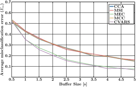
The same non-overlapping EEG segments from sec-tion 5.1 were used to compare the CCA, MCC, MSI, MEC and CVARS methods. The mean misclassifica-tion error averaged over all subjects is shown in
fig-ure 12 forNh= 3 andFs= 512 Hz. MEC and CVARS
were used with AR(7) model. By visual inspection, the results of the CCA, MCC and MSI methods don’t differ significantly. The MEC and CVARS methods outper-form CCA for all buffer lengths, except for 0.5 s buffers, in which case, all methods have comparable accuracies. The CVARS method performs slightly better than the MEC for almost all buffer lengths.
Furthermore, the upper three rows in figure 13 compare the CCA, MEC and CVARS with respect to their score evolution during the first full stimulation
sequence with (N, T) = (1024,1) samples. CVARS
ρ1
P
(
ρ1
)
5 10
15 15.0 Hz12.0 Hz
10.0 Hz 8.57 Hz
P
(
ρ
2
)
ρ2
5 10 15
P
(
ρ3
)
ρ3
5 10 15
P
(
ρ4
)
ρ4
5 10 15
P
(
ρ5
)
ρ5
5 10 15
P
(
ρ6
)
5 10 15
[image:12.612.63.495.60.316.2]0 0.1 0.2 0.3 0.4 0.5 0.6 0.7 0.8 0.9 1
Figure 10: Distribution of target (solid) and nontarget (dotted) canonical correlations averaged over all subjects from overlapping EEG segments. For instance, the distributions of target ρi forf1 = 15 Hz were obtained by
computing the canonical correlations of EEG segmentsY∈R1024×16 whereg(Y) =f
1 withscca(Y,Xf1). The
nontarget distributions were obtained from segments withg(Y)6=f1.
Buffer Size [s]
A
v
e
ra
g
e
m
is
c
la
ss
i
fi
c
a
ti
o
n
e
rr
o
r
(
Em
)
0.1 0.2 0.3 0.4 0.5 0.6 0.7
0.5 1 1.5 2 2.5 3 3.5 4 4.5 5
CCA MSI MEC MCC CVARS
Figure 12: Average misclassification accuracy
averaged over all frequencies and subjects. As
expected, classification accuracies for CCA (plotted with thick line to highlight this fact) and MCC are the same.
for the stimulation frequency f1 = 15 Hz and less
for f2 = 12 Hz. Less or no improvement can be
observed for the subject with the high SNR (S5).
From the score evolution (N = 1024, T = 1) data,
we have computed the average accuracy per subject over all stimulation frequencies (excluding the idle state) for the unsupervised CCA, standard MEC and CVARS. A repeated measures ANOVA determined
that mean classification accuracy differed statistically
significantly between the three methods (F(2,18) =
19.902, p <0.0001,partialη2 = 0.689). Post hoc tests
using the Bonferroni correction revealed statistically
significant (p = 0.005) improvement of unsupervised
CVARS (mean±std: 0.739±0.099) over unsupervised
CCA (mean± std: 0.64 ± 0.137). Furthermore, we
found a trend for unsupervised CVARS being superior over unsupervised standard MEC, which given the current number of subjects though is not significant
(p = 0.069). Unsupervised standard MEC (mean±
std: 0.72±0.107) performed significantly better than
the unsupervised CCA (p= 0.003).
The effect of choosing longer buffers (N = 2560)
with CVARS method is shown in the lower panel of figure 13. We can easily observe that fluctuations in the score function are reduced for bothS2 andS5, with the side effect of introducing delays into the system (rise-up and decaying delays). This, however, did not
guarantee reliable SSVEP detection forS2.
5.4. Supervised CVARS method for SSVEP detection
[image:12.612.60.281.392.533.2]Time [s] sc
c
a
Subject: 5, Method: CCA, (N,T)=(1024,1)
0 0.1
0.2
0.3
0.4
0.5
0.6
0.7
0.8
0.9
1
5 10 15 20 25 30 35 40 45 50 55 15.0 Hz
12.0 Hz 10.0 Hz 8.57 Hz Trigger
Time [s] sc
c
a
Subject: 2, Method: CCA, (N,T)=(1024,1)
0 0.1
0.2
0.3
0.4
0.5
0.6
0.7
0.8
0.9
1
5 10 15 20 25 30 35 40 45 50 55 15.0 Hz
12.0 Hz 10.0 Hz 8.57 Hz Trigger
Time [s]
sm
e
c
Subject: 5, Method: MEC, (N,T)=(1024,1)
0 2 4 6 8 10 12 14 16
5 10 15 20 25 30 35 40 45 50 55
15.0 Hz 12.0 Hz 10.0 Hz 8.57 Hz Trigger
Time [s]
sm
e
c
Subject: 2, Method: MEC, (N,T)=(1024,1)
0 2 4 6 8 10 12 14 16
5 10 15 20 25 30 35 40 45 50 55
15.0 Hz 12.0 Hz 10.0 Hz 8.57 Hz Trigger
Time [s]
sc
v
a
r
s
Subject: 5, Method: CVARS, (N,T)=(1024,1)
0 10 20 30 40 50 60 70 80
5 10 15 20 25 30 35 40 45 50 55
15.0 Hz 12.0 Hz 10.0 Hz 8.57 Hz Trigger
Time [s]
sc
v
a
r
s
Subject: 2, Method: CVARS, (N,T)=(1024,1)
0 10 20 30 40 50 60 70 80
5 10 15 20 25 30 35 40 45 50 55
15.0 Hz 12.0 Hz 10.0 Hz 8.57 Hz Trigger
Time [s]
sc
v
a
r
s
Subject: 5, Method: CVARS, (N,T)=(2560,1)
0 20 40 60 80 100 120
5 10 15 20 25 30 35 40 45 50 55
15.0 Hz 12.0 Hz 10.0 Hz 8.57 Hz Trigger
Time [s]
sc
v
a
r
s
Subject: 2, Method: CVARS, (N,T)=(2560,1)
0 20 40 60 80 100 120
5 10 15 20 25 30 35 40 45 50 55
[image:13.612.65.546.61.643.2]15.0 Hz 12.0 Hz 10.0 Hz 8.57 Hz Trigger
Figure 13: Score evolution for S5 (left) and S2 (right) obtained during the first stimulation sequence of the first recording session for buffers of 2 seconds (except for the last row this was 5 s),T = 1 sample and Nh= 3 with the CCA, MEC, and CVARS methods. AR(7) models were used when necessary. The trigger is shown as a staircase with 4 levels, each level corresponds to one stimulation frequency. For example, level 2 corresponds tof2= 12 Hz. The zero level corresponds to the idle state. The fourth level (i.e. forf4) is scaled to the largest
figures 10 and 13 suggest that the simple argmax function in (5) will provide faulty detections due to the large visible difference in the mean scores for the different driving frequencies, and the resulting bias
towards the lower frequencies. Learning a simple
threshold from labeled data (obtained from a training session for each user), although can reduce the rate of false alarms and faulty detections, can lead also to a larger rate of misses as can easily be seen for CCA from the plots in figure 10 and for all methods in figure 13. For instance setting a CCA threshold of 0.5 in figure 10 would result in a high probability of miss, as can be computed from the area under the curves of the target distributions for ρ1 < 0.5. It
can be additionally observed that it is more probable to miss the detection of higher frequencies than the lower ones. Linear Discriminant Analysis (LDA) lends itself naturally to such a problem, where labeled score vectors are obtained from one training session and an LDA classifier is thereby learned. In online sessions, the scores are computed as usual to produce the vector
s ∈ RNf×1. The LDA classifier is then applied on s
to provide the final estimate of the hidden attended stimulus. We summarize the comparison between the
unsupervised and supervised CVARS with (N, T) =
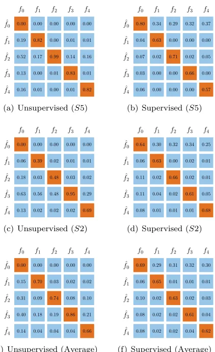
(1024,128) in the form of the confusion matrices shown in figure 14, for subjectsS5 andS2, in addition to the average over all subjects. We chose CVARS here as it provided the best results in the unsupervised case. The confusion matrices were computed with each method applied on the two available recording sessions. In case of the supervised CVARS, a classifier was learned from each session and applied on the other one, and results therefrom were averaged (i.e. a total of two classifiers were used per subject). These results clearly show a reduction in the rate of false alarms on the expense of higher probability of misses. The probability of miss and that of correct detections are quite uniform with respect to the stimulation frequencies, on the contrary to what is expected if a single threshold were used. Furthermore, a large portion of the probability of miss in the supervised CVARS replaces some of the wrong detections in the unsupervised case. Falsely detecting one control state as the idle state is generally favored over confusing it with another control state.
5.5. Discussion
From the results in the previous subsections, we can see that there are conflicting factors that affect the detection accuracy of SSVEP. On one hand, accuracy is a monotonically increasing function of the buffer size (i.e. N), should the buffer contain only homogeneous data, which is not the most probable case in online applications. On the other hand, larger buffer sizes introduce delays, as the old samples which contain no
f0 f1 f2 f3 f4
ˆ
f0 0.00 0.00 0.00 0.00 0.00
ˆ
f1 0.19 0.82 0.00 0.01 0.01
ˆ
f2 0.52 0.17 0.99 0.14 0.16
ˆ
f3 0.13 0.00 0.01 0.83 0.01
ˆ
f4 0.16 0.01 0.00 0.01 0.82
(a) Unsupervised (S5)
f0 f1 f2 f3 f4
ˆ
f0 0.80 0.34 0.29 0.32 0.37
ˆ
f1 0.04 0.63 0.00 0.00 0.00
ˆ
f2 0.07 0.02 0.71 0.02 0.05
ˆ
f3 0.03 0.00 0.00 0.66 0.00
ˆ
f4 0.06 0.00 0.00 0.00 0.57
(b) Supervised (S5)
f0 f1 f2 f3 f4
ˆ
f0 0.00 0.00 0.00 0.00 0.00
ˆ
f1 0.06 0.39 0.02 0.01 0.01
ˆ
f2 0.18 0.03 0.48 0.03 0.02
ˆ
f3 0.63 0.56 0.48 0.95 0.29
ˆ
f4 0.13 0.02 0.02 0.02 0.69
(c) Unsupervised (S2)
f0 f1 f2 f3 f4
ˆ
f0 0.64 0.30 0.32 0.34 0.25
ˆ
f1 0.06 0.63 0.00 0.02 0.01
ˆ
f2 0.11 0.02 0.66 0.02 0.01
ˆ
f3 0.11 0.04 0.02 0.61 0.05
ˆ
f4 0.08 0.01 0.01 0.01 0.68
(d) Supervised (S2)
f0 f1 f2 f3 f4
ˆ
f0 0.00 0.00 0.00 0.00 0.00
ˆ
f1 0.15 0.70 0.03 0.02 0.02
ˆ
f2 0.31 0.09 0.74 0.08 0.10
ˆ
f3 0.40 0.18 0.19 0.86 0.21
ˆ
f4 0.14 0.04 0.04 0.04 0.66
(e) Unsupervised (Average)
f0 f1 f2 f3 f4
ˆ
f0 0.69 0.29 0.31 0.32 0.30
ˆ
f1 0.06 0.65 0.01 0.01 0.01
ˆ
f2 0.10 0.02 0.63 0.02 0.03
ˆ
f3 0.08 0.02 0.02 0.61 0.04
ˆ
f4 0.08 0.02 0.02 0.04 0.62
[image:14.612.325.536.62.407.2](f) Supervised (Average)
Figure 14: Confusion matrices for the unsupervised
and supervised CVARS methods. The supervised
CVARS method produces reliable results for all
participants includingS2, whose data has been shown
to have low SNR. This proves the ability of supervised CVARS to deal with wide range of SNR levels.
information about the currently attended stimulus still
inhabit the buffer Y and contribute to the different
values s(Y,Xf), leading to false alarms and faulty detections.
Comparing figures 6 and 15, which respectively show the misclassification results of non-overlapping segments as a function of buffer length for CCA (Nh=
1) and CVARS (Nh = 3), we can see that buffer
lengths, at which acceptable accuracies are obtained, differ from one subject to another, regardless of the detection method used. Therefore, a trade-off between accuracy and speed should be optimized for each subject, based on a short training session. The same session is also used to learn the LDA classifier from the obtained scores.
Buffer Size [s]
A
v
e
ra
g
e
m
is
c
la
ss
i
fi
c
a
ti
o
n
e
rr
o
r
(
Em
)
0.1
0.2
0.3
0.4
0.5
0.6
0.7
0.5 1 1.5 2 2.5 3 3.5 4 4.5 5
S1 S2
S3 S4
S5 S6
S7 S8
S9 S10
mean
Figure 15: Average CVARS-method misclassification error computed as a function of buffer length for non-overlapping segments.
ρ
f
(
ρ
)
0
.002
0.006
0
.01
0.014
0.018
0 0.1 0.2 0.3 0.4 0.5 0.6 0.7 0.8 0.9 1
f(ρ)
q(ρ) =ρ2/66
Figure 16: The functionf(ρ) qualitatively shows the relatively large contribution of the maximum canonical correlation in the final MSI score, especially when ρ1>0.5. Forρ1≤0.5, smsi≈P2i=1Nhρ2i.
give exactly the same estimates and thus the same misclassification error rates. MSI and CCA have shown similar misclassification error rates, suggesting thatρ1
plays a major role in calculatingsmsi. This can be seen
by rewriting (13) assmsi=P2i=1Nhf(ρi), where
f(ρ) = (1 +ρ) log(1 +ρ) + (1−ρ) log(1−ρ)
Plog(P) . (20)
Figure 16 plotsf(ρ) in the range of [0,1] in addition to the functionq(ρ) =ρ2/C, whereC is a constant. The
quadratic function q(ρ) approximates f(ρ) relatively well when ρ < 0.5. Therefore, for the case when all ρi < 0.5, the MSI score function (and its quadratic approximation) gives more weight to greater ρi’s. On the other hand, when ρ1 > 0.5, the contribution of
ρ1becomes more emphasized as the differencef(ρ1)−
q(ρ1) grows very rapidly. The latter case is the more
probable case given the empirical values of targetρi’s shown in figure 10.
Furthermore, we have shown that MEC outper-forms CCA. This result differs from what was shown
in [34]. However, the score function smec used there
was defined with ˆσkl = 1, which ignores the noise power at the stimulation frequencies and consequently MEC scores will be biased towards the low frequencies. This reaffirms the need to scale the different correlations with regard to estimates about the noise power, which is done efficiently with test statistics used in standard MEC and CVARS procedures. In [15], a test statis-tic similar tosmec is used with the MCC spatial filter,
where the spatial filter is obtained from a subset of the columns inWy. Again, this statistic should give simi-lar results to the CVARS when the data is pre-whitened before applying the MCC filter.
Alternatively, Yin et al. [35] proposed the
supervised CCA-RV method for the same purpose of reducing the variability in the final target scores of the different stimulation frequencies wherescca-rv was
computed with
scca-rv(Y,Xf) =
scca(Y,Xf)−scca-nt(Y,Xf) scca(Y,Xf) +scca-nt(Y,Xf)
, (21)
wherescca-nt(Y,Xf) is the mean nontarget scores of a
frequency f computed from a training session. Since
the CCA-RV method was published very recently, we could not fully and fairly compare it to the CVARS method, especially also that real-time biofeedback
mechanisms were employed in [35]. However, we
claim that the supervised CVARS method described in this paper should outperform the supervised CCA-RV (when we ignore the effect of the biofeedback). Firstly, CVARS has been shown in the current paper to outperform CCA when results for all subjects were averaged and therefore plugging the CVARS scores instead of CCA in (21) is expected to provide, on average, better results. Additionally, LDA learns from the available training session the optimal mapping from the CVARS scores to the stimulation frequencies as it takes into account not only the mean values as it is the case in [35] but also the variances and covariations of the individual scores.
Throughout this work, we had a number of
channels Ny = 16, which was larger than the number
of signals assumed in the source modelNx= 2Nh= 6. Reversing this relation does not affect the obtained results. For the CCA method, the number of canonical correlations is upper bounded by min(Nx, Ny), which
will be Ny in this case. The eigenvalues in the MSI
[image:15.612.61.278.61.197.2] [image:15.612.61.279.256.393.2]comparable to 2Nh= 4. For our dataset, we got typical values of Ns ∈ {14,15,16} for Ny = 16 and Nh = 3. The result we proved here regarding the conditions
whenWMEC =W0y makes the CVARS method more
consistent with the assumptions about the the number of source model signals.
6. Conclusion
Detection of SSVEP in continuous EEG signals lies under the general problem of detecting sinusoids in noisy measurements, a problem that has been thoroughly investigated in the array signal processing field. We have theoretically shown the conditions in which state-of-the-art SSVEP detection methods share similar spatial filters, a step required to enhance the overall signal-to-noise ratio. The equivalence of the discrimination power of the MCC and CCA methods has been proven and it was conjectured that MSI
should have very similar results as well. Empirical
evaluations supported these results. The methods
CCA, MCC and MSI rely on a single metric that
is computed from the canonical correlations ρi to
provide an estimate about the stimulation frequency,
to which a user is attending. Thereby they fail to
provide reliable estimates when the signal is lost in the noise floor. The MEC and the hereby proposed CVARS methods, in addition to the step of spatial filtering, base their discrimination upon the estimated signal and noise powers at each considered frequency (the fundamental stimulation frequency and its higher
harmonics). We have shown that the CVARS and
the MEC scores are the same, given that the EEG signal is spatially whitened before running MEC algorithm andNs is rather fixed to min(Ny,2Nh), i.e. number of canonical correlations. The CVARS method slightly outperformed the standard MEC method, which typically requires no spatial pre-whitening as
reported in [15]. Finally, we have shown that the
supervised CVARS method based on a short training session can be used to learn a mapping function rather than the maximizer (argmax) that estimates the hidden driving frequency and the idle state from the obtained scores, reliably and accurately. The training session should also serve the purpose of finding the optimal buffer size for a specific subject to be used in online applications.
Acknowledgments
This work is supported in part by the VERE project within the 7th Framework Programme of the European Union, FET-Human Computer Confluence Initiative, contract number ICT-2010-257695 and the Institute for Advanced Study, Technical University of Munich
(TUM).
Appendix A. Relation between MSI and CCA
Finding the eigenvalues of the matrix R defined
in (12) involves solving the characteristic equation det(R−λI) = 0, and thus
det
INx−λINx T TT INy −λINy
= 0
Without loss of generality, we assume in the following thatNy≥Nx. Using the Schur determinant identity we can write
0 = det INy −λINy
·det
(1−λ)INx− 1
1−λTT
T
= (1−λ)Ny ·det
1
1−λ
(1−λ)2INx−TTT
= (1−λ)Ny · 1
(1−λ)Nx ·det
(1−λ)2INx−TTT
= (1−λ)Ny−Nx·det(1−λ)2INx−TTT
,
which means that either λ = 1 or (1 −λ)2 is one
of the eigenvalues of TTT. Consequently, there are
exactly (Ny−Nx) eigenvalues ofRthat take the value 1. The remaining 2Nxeigenvalues can be related to the canonical correlations (subsection 3.1) withλ= 1∓ρi, wherei= 1, . . . , Nx.
References
[1] Ken Nakayama and Manfred Mackeben. Steady state visual evoked potentials in the alert primate. Vision Research, 22(10):1261–1271, 1982.
[2] Christoph S Herrmann. Human EEG responses to 1-100 Hz flicker: Resonance phenomena in visual cortex and their potential correlation to cognitive phenomena.
Experimental Brain Research, 137(3-4):346–353, apr
2001.
[3] Athanasios P Liavas, George V Moustakides, G¨unter Henning, Emmanuil Z. Psarakis, and Peter Husar. A periodogram-based method for the detection of steady-state visually evoked potentials. IEEE Transactions on Biomedical Engineering, 45(2):242–248, 1998.
[4] Almudena Capilla, Paula Pazo-Alvarez, Alvaro Darriba, Pablo Campo, and Joachim Gross. Steady-state visual evoked potentials can be explained by temporal superposition of transient event-related responses. PloS one, 6(1):e14543, 2011.
[5] S. T. Morgan, J. C. Hansen, and S. A. Hillyard. Selective attention to stimulus location modulates the steady-state visual evoked potential. Proceedings of the National
Academy of Sciences of the United States of America,
93(10):4770–4774, may 1996.
[6] Yu Te Wang, Yijun Wang, Chung Kuan Cheng, and Tzyy Ping Jung. Developing stimulus presentation on mobile devices for a truly portable SSVEP-based BCI.