Psychologically inspired dimensionality reduction for 2D and 3D Face Recognition

Psychologically inspired dimensionality reduction

for 2D and 3D Face Recognition

Mark F. Hansen, Gary A. Atkinson,

Melvyn L. Smith, Lyndon N. Smith

The Machine Vision Laboratory

University of the West Of England

Bristol, UK

Abstract

We present a number of related novel methods for reducing the dimen-sionality of data for the purposes of 2D and 3D face recognition. Results from psychology show that humans are capable of very good recognition of low resolution images and caricatures. These findings have inspired our experiments into methods of effective dimension reduction. For experi-mentation we use a subset of the benchmark FRGCv2.0 database as well as our own photometric stereo “Photoface” database. Our approaches look at the effects of image resizing, and inclusion of pixels based on per-centiles and variance. Via the best combination of these techniques we represent a 3D image using only 61 variables and achieve 95.75% recog-nition performance (only a 2.25% decrease from using all pixels). These variables are extracted using computationally efficient techniques instead of more intensive methods employed by Eigenface and Fisherface tech-niques and can additionally reduce processing time tenfold.

1

Introduction

Automatic face recognition has been an active area of research for over four decades and a key part of this research is understanding how different data representations affect recognition rates and efficiency. Digital images of faces

have a very high data dimensionality: a 200×200px image defines a point in

In this paper, we prove the following contributions for both the FRGCv2.0 database [1] and our own photometric stereo database [2] captured using the “Photoface” device [3]:

1. Optimal recognition results for close-cropped faces are obtained when the resolution is reduced to a mere 10x10 pixels.

2. The exclusive use of just 10% of the data (chosen to be those pixel locations with the greatest variance) is sufficient to maintain recognition rates to within 10% of those rates that include all of the data.

3. When combining the above two contributions we perform recognition at an accuracy of 96.25% for 40 subjects using only 61 dimensions (pixels). This compares to 98% when the full 80x80 resolution is used on all data.

Ultimately we aim to compare dimension reduction techniques based on a percentile and variance based inclusion principle (to exclude 90% of the data) with a baseline condition containing all pixels.

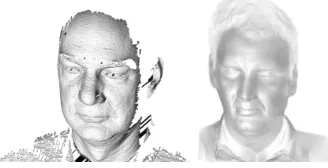
Our own database, Photoface, provides over 3000 sessions of 457 individuals, and scans are captured using photometric stereo [4] which results in estimated surface normals at each pixel. Full details of the actual device used can be found in [3] and an example of a scan can be seen in Fig. 1. The FRGCv2.0 database, which we also use in this paper, does not provide the surface normals. They can be calculated by numerically differentiating the point cloud data. We also include experiments on the depth map images to rule out any errors introduced by differentiation.

Figure 1: Examples of FRGCv2.0 (left) and Photoface (right) 3D scans. NB They are not of the same person.

Using 3D data for face recognition allows for pose and illumination correction

which are two commonly

cited problems with

conven-tional 2D images. Better

recognition rates have also been reported using 3D over 2D data [5], although this is not always replicated [6]. One reason for this may be the representation of the 3D data

used in the analysis. G¨okberk

et al.[7] performed

recogni-tion experiments using numerous 3D representarecogni-tions. They concluded that

‘. . . surface normals are better descriptors than the 3D coordinates of the facial points.’ This is at odds with most research which uses the 3D point coordinates as a starting point. Surface normals are used in the experiments performed in this paper for this reason.

techniques are commonly used in face recognition. With an added dimension, 3D face models potentially compound the problem for large data storage. Recent techniques such as sparse representation (such as non-negative matrix factor-ization) and manifold learning (such as local linear embedding [10]) show that effective methods of dimension reduction are a key topic. Methods that can reduce the amount of data without discarding discriminatory information are essential for faster processing and optimal solutions. There have been many at-tempts in the literature to extend and generalise PCA, FLD and other methods [11, 12, 13] in order to improve robustness to pose, illumination, etc, typically at the expense of computational efficiency. The main contribution of this paper by contrast, is to show that for the constrained case of frontal 2.5D data, then the efficiency can be improved even compared to PCA by using more direct analysis without the need to project into a new subspace.

Caricaturing essentially enhances those facial features that are unusual or deviate sufficiently from the norm. It has been shown that humans are better able to recognise a caricature than they are the veridical image [14, 15]. This finding is interesting as caricaturing is simply distorting or adding noise to an image. However this noise aids human recognition and this, in turn, provides insights into the storage or retrieval mechanism used by the human brain.

Unnikrishnan [16] conceptualises an approach similar to face caricatures for human recognition. In this approach, only those features which deviate from the norm by more than a threshold are used to uniquely describe a face.

Unnikrish-nan suggests using those features whose deviations lie below the 5th_percentile

and above the 95th_{percentile, thereby discarding 90% of the data.}

Unnikrish-nan provides no empirical evidence in support of his hypothesis, so an aim of this paper is to test the theory experimentally. We do this in two ways: the first directly tests his theory, finding the thresholds for each pixel which represent

the 5th _{and 95}th _{percentile values and only including those pixels in each scan}

which lie outside them (outliers). The second is loosely based on Unnikrishnan’s idea, and looks at the variance across the whole database to calculate the pixel locations with the largest variance. Only the pixels at these locations are then used for recognition.

An obvious method of reducing the amount of data is to downscale the im-ages. A great deal of research has gone into increasing the resolution of poor quality images (super-resolution [17, 18], hallucinating [19]) by combining im-ages or using statistical techniques to reproduce a more accurate representation

of a face (e.g.from CCTV footage). By contrast, little research attempts to

directly investigate resolution as a function of recognition rates on 3D data.

Todericiet al.state that there is little to be gained from using high resolution

images [20], Boomet al.state that the optimum face size is 32×32 px for

regis-tration and recognition [21], a view which is reinforced by a more recent study

by Luiet al.who state that optimum face size lies between 32 and 64 pixels [22].

These experiments have used 2D images. Changet al.use both 2D and 3D data

algorithms). These findings are conducive to the fact that the same appears to be true of human recognition [23].

2

Methods and data

This section details the datasets, preprocessing steps, and the methods used in the experiments.

2.1

Data and preprocessing

Experiments were performed on 10 sessions of 40 subjects facing frontally with-out expression on the FRGCv2.0 and our own photometric stereo database. 2D and 3D data are used in separate experiments.

The FRGCv2.0 dataset comes in point cloud format which is converted to a mesh via uniform sampling across facets. Noise is removed by median smoothing and holes filled by interpolation. Normals are then estimated by differentiating the surface. The depth map images are all normalized to have a minimum value of 0.

+ +

d

d/20 d/20 d/3

d

d

Figure 2: The cropped

region of a face. The

distance between the

anterior canthi (d) is used to calculate the cropped region.

Data is cropped for both databases as follows: the median anterior canthi and nose tip across all ses-sions are used for alignment via linear transforms. The aligned images are then cropped into a square region as shown in Fig. 2 to preserve main features of the face (eyes, nose, mouth), and exclude the forehead and chin regions which can frequently be occluded by hair.

Our 2D experiments are based on data as follows: the accompanying colour image for each FRGCv2.0 scan is converted to greyscale, aligned and cropped in the same way as the 3D scan. The 2D images in the Photoface database are the estimated albedo images which are also aligned and cropped in the same way as the 3D data. Due to memory limitations, both the

2D and 3D data are then resized to 80×80 px and are

reshaped into a 6400-dimension and a 12800-dimension (x and y components of the surface normals are concatenated) vector respectively.

2.2

Calculating outliers and variance

The thresholds for each pixel are calculated which represent the 5th _{and 95}th

percentile values. We are interested in the norm across the whole dataset for each pixel location rather than the norm for each image. For the 2D images, percentile values are calculated for the greyscale intensity value for each pixel location. There are 400 sessions, so there are 400 values for each pixel from which we calculate the percentile thresholds. The same process is performed for

for each pixel. Pixels which have a value between the 5th and 95th percentile are discarded, leaving only the 10% outlying data. We shall refer to this as the “percentile inclusion criterion”. Examples can be seen in Fig. 3.

Figure 3: Examples of they-components of the surface

normals that have values outside the 5th_{and 95}th

per-centiles for four subjects which are used for recognition.

The above method extracts the least com-mon data from each session and that is what is used for

recog-nition. Alternately,

we can use the greyscale variance at each pixel location as a

mea-sure of

discrimina-tory power. If a pixel shows a large variance across the dataset, then this

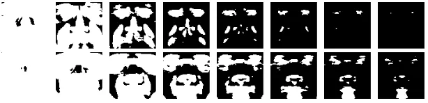
might make it useful for recognition (assuming that variance within the class or subject is small). Therefore the standard deviation of each pixel is calcu-lated over all the sessions. Whether or not a particular pixel location is used in recognition depends on whether or not the variance is above a pre-determined threshold. Examples of the use of different thresholds are shown in Fig. 4. We refer to this as the “variance inclusion criterion”.

Figure 4: Examples of the regions which remain for x (top row) and

y-components (bottom row) as the threshold variance is increased from left to right. White regions are retained and black regions are discarded.

2.3

Image resizing

The effect of different resizing techniques on linear subsampling are investigated in terms of their effect on recognition as a function of resolution. Resizing is

performed via the Matlabimresize()function using the deafult bicubic kernal

type and with antialiasing on, as these settings were found to provide the best performance.

2.4

Recognition algorithm

As the purpose of this research is feature extraction efficiency, the actual choice of classifier is not so important. We therefore implement Pearson product-moment correlation coefficient (PMCC) as a similarity measurement between a probe vector and the gallery vectors. The gallery session with the highest coefficient is regarded as a match. Experimentally, we found that PMCC gives similar performance on baseline conditions to the Fisherface algorithm but is approximately eight times faster.

3

Results

3.1

Dimensionality reduction via the percentile inclusion

criterion

Unnikrishnan’s theory states that we should expect reliable performance using

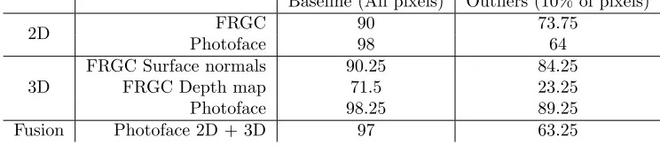
only the data which lies outside the 5th_{and 95}th_{percentiles [16]. Table. 1 shows}

recognition rates on 2D and 3D data using both all data and the outliers only. Note in particular that, for the 3D surface normal data, the rates drop by under 10% when using outlier data only. This effect seems limited to the surface normal data and is not seen in either the 2D or depth map data. We have included results from a fusion technique using the Photoface surface normal data combined with the albedo image. There is a small decrease in baseline performance and using only the outlying data leads to a severe decrease of about 34%.

Baseline (All pixels) Outliers (10% of pixels)

2D FRGC 90 73.75

Photoface 98 64

3D

FRGC Surface normals 90.25 84.25

FRGC Depth map 71.5 23.25

Photoface 98.25 89.25

Fusion Photoface 2D + 3D 97 63.25

Table 1: Baseline versus outlier performance (% correct).

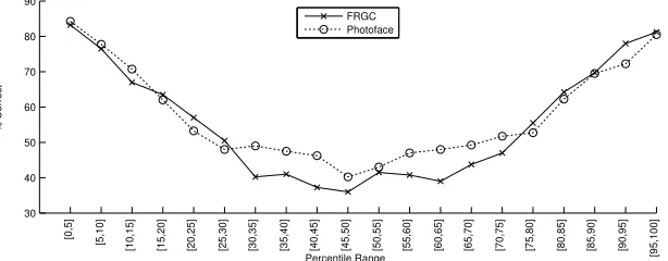
Fig. 5 shows a plot of recognition rate as a function of which percentile range is used for recognition on 3D Photoface data. It should be noted that similar patterns of results were found for all datasets (2D, 3D and FRGC). As predicted, the figure shows that the best recognition performance is obtained

using the most outlying percentiles. As expected also, the recognition rate

reduces as the percentile ranges used tend toward the inliers. However, for the most inlying data of all (i.e. percentiles 45–55) we find a significant increase in performance. Contrary to Unnikrishnan’s theory, this implies that there is discriminative data that is useful for face recognition in the most common data as well as the most outlying.

In a related experiment, we used single 5% ranges of data for recognition

20 30 40 50 60 70 80 90

Percentile ranges used for recognition (Lower, Upper)

% Correct

0−5,95−100 5−10,90−9510−15,85−9015−20,80−8520−25,75−8025−30,70−7530−35,65−7035−40,60−6540−45,55−6045−50,50−55 FRGC

Photoface

Figure 5: Recognition performance using pairs of percentile ranges for 3D data.

recognition performance for the most inlying data is not replicated. The slightly lower performance compared with Fig. 5 is because only 5% of the data is used instead of 10%.

Performance increases by combining ranges are not always observed.

Con-sider, for example, the 25−30th _{and 70−75}th _{percentiles for the FRGCv2.0}

data. Individually the two percentiles give a performance around the 50% mark in Fig. 6, but when combined, the performance drops to around 40% in Fig. 5.

30 40 50 60 70 80 90

Percentile Range

% Correct

[0,5] _[5,10]

[10,15] [15,20] [20,25] [25,30] [30,35] [35,40] [40,45] [45,50] [50,55] [55,60] [60,65] [65,70] [70,75] [75,80] [80,85] [85,90] [90,95] _[95,100] FRGC

Photoface

Figure 6: FRGC and Photoface data show a marked symmetry across ranges of percentiles.

3.2

Dimensionality reduction via the variance inclusion

criterion

using the percentiles defined within a single image as an inclusion criterion, we use the variance of a particular pixel across all subjects as explained in Sec. 2.2. Fig. 7 shows plots combining the number of pixels which remain as we remove those with least variance (bar plot) against the recognition performance (line plot). It is apparent that we can achieve close to optimal performance while losing a large proportion of the pixels. We can discard approximately 75% of the least varying pixels and observe a corresponding drop of less than 10% in recognition performance on the FRGC data. Indeed, for Photoface data specifically, we only lose a few percent.

2D 3D

FRGC

30 40 50 60 70 80

0 1000 2000 3000 4000 5000 6000 7000 Variance Threshold Pixels % Correct 40 50 60 70 80 90

0.1 0.2 0.3 0.4 0.5 0 2000 4000 6000 8000 10000 12000 14000 Variance Threshold Pixels % Correct 20 30 40 50 60 70 80 90 100 Photoface

20 25 30 35 40 45

0 1000 2000 3000 4000 5000 6000 7000 Variance Threshold Pixels % Correct 65 70 75 80 85 90 95 100

0.05 0.1 0.15 0.2 0.25 0.3 0 2000 4000 6000 8000 10000 12000 14000 Variance Threshold Pixels % Correct 70 75 80 85 90 95 100

Figure 7: Recognition (line) as a function of retained pixels (bar chart). The pattern is shown in both sets of data (FRGC on the top row and Photoface on the bottom). 2D (grayscale for FRGC and albedo for Photoface) on the left, and surface normal data is shown on the right.

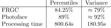
Table 2 shows a performance comparison of the two types of inclusion criteria when only 10% of pixels are retained. It is clear that by discarding the data that varies the least, we can maintain reasonably high recognition rates.

Percentiles Variance

FRGC 84.25% ≈79%

Photoface 89% ≈92%

Processing time 800.64s 180.95s

Table 2: A comparison of recognition performance using percentiles and vari-ance methods to select the most discriminatory 10% of the data. The processing time includes the calculation of the outliers/most varying pixels and 400 classi-fications

decreased the vector size by 90 %. This compares to 973.09s for the equivalent Fisherface analysis which provides an accuracy of 99.5% so both methods offer considerable time savings at a small cost to accuracy.

3.3

Optimisation of Image resolution

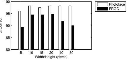
Finally the effect of image resolution on 3D recognition performance is shown

in Fig. 8. This clearly shows that a resolution of 10×10 px provides optimal

or close to optimal recognition performance (the result for 40×40 px is 0.25%

higher for FRGC) on both 3D datasets. The same pattern appears in the 2D Photoface database, but there is a small decrease of just under 3% for the 2D

FRGC data. Nonetheless, if we take the 10×10 px as an optiumum size, this

figure is lower than often reported in the literature. This may be because the data used in these experiments is already highly cropped, and other research may be using other metrics such as the distance across the uncropped head. Although not shown in the figure, not antialiasing the resampled images led to poorer performance in all cases.

5 10 15 20 40 80

80 85 90 95 100

Width/Height (pixels)

% Correct

Photoface FRGC

Figure 8: The effect of resolution on 3D recognition performance. Recognition

rates for 10×10 px are 94.75% for FRGC data and 98.25% for Photoface data.

Combining the optimal resolution of 10×10 px with the variance method

above we can achieve virtually the same recognition performance as an 80×80 px

image but using only 64 pixels for FRGC data and 61 pixels for Photoface data. Recognition rates of 87.75% and 96.25% are recorded (a loss of only 7% and 2% respectively). The processing time is also reduced to 10.5s for variance analysis and 400 classifications. The same analysis using the Fisherface algorithm takes 118s and achieves a comparable rate of 89.25%.

4

Discussion

commonly used dimension reduction techniques of PCA and Fisherface with our variance and percentile inclusion criterion techniques at different resolutions in terms of classification accuracy and processing time. All experiments were car-ried out in Matlab on a Quad Core 2.5GHz Intel PC with 2GB ram running Windows XP. Only one percentile inclusion criterion result has been included as performance (especially processing time) was not at the same level as other conditions.

Res. (px) Data Reduction Classifier No. Dimensions % Correct Proc. time(s)

1. 10x10 None PMCC 200 98.25 12.02

2. 10x10 VI PMCC 19 (10%) 82.75 12.52

3. 10x10 VI PMCC 61 95.75 13.02

4. 10x10 PCA Euc. dist. 21 94.5 92.47

5. 10x10 PCA PMCC 21 92.25 97.16

6. 10x10 61PCA Euc. dist. 61 96.25% 102.91

7. 10x10 VI→15PCA PMCC 61→15 89.75 128.54

8. 10x10 VI→FF Euc. dist. 19→19 90.5 129.74

9. 80x80 None PMCC 12800 98.25 129.86

10. 10x10 VI→15PCA PMCC 19 (10%)→15 79 132.56

11. 10x10 VI→FF Euc. dist. 61→39 99 134.69

12. 10x10 FF Euc. dist. 39 100 144.25

13. 80x80 VI PMCC 1235 (10%) 92.25 180.95

14. 80x80 VI→15PCA PMCC 1235 (10%)→15 85.25 331.40

15. 80x80 VI→FF Euc. dist. 1235 (10%)→39 90.75 549.25

16. 80x80 PCA Euc. dist. 61 96.75 573.52

17. 80x80 PI PMCC 12800 89 800.64

18. 80x80 FF Euc. dist. 39 99.5 973.09

Table 3: A comparison of our variance (VI) and percentile (PI) inclusion tech-niques with PCA and Fisherface (FF) algorithms sorted by processing time.

The number of components which are used for PCA depends on the specific test as follows: 61 components (61PCA, row 6 of Table 3) were chosen for a direct comparison with the 61 variables of the variance inclusion criterion which gave good performance in Fig. 7. 15 components (15PCA condition, rows 7, 10 & 14) were chosen arbitrarily as an extra step after the variance inclusion criterion for its low dimensionality and relatively good performance. For other tests using PCA, the number of components are chosen which describe 85%

of the variance. Some entries in the “No. Dimensions” column have (10%)

shown next to them. This is a reminder that only 10% of the data remains after applying the variance inclusion criterion. Finally some of the rows contain

a “→” symbol representing a combination of processes eg Variance Inclusion

followed by Fisherface.

Generally resizing the image to 10x10 pixels gives a clear processing time advantage with little or no compromise on accuracy. Without additional dimen-sionality reduction we achieve a recognition rate of 98.25% (row 1). We are able

to reduce the dimensionality by a further 2₃ and only lose 2.5% performance by

(row 3). This appears to give the best compromise in terms of the number of dimensions, processing time and accuracy . The Fisherface algorithm gives ex-cellent performance (10x10 Fisherface gives 100% accuracy, row 12) but at the cost of processing time.

These results only apply to the simplest case in face recognition – the frontal, expressionless face. The variance inclusion algorithm would be unlikely to pro-duce similarly good results if expressions were present in the dataset, as these are likely to produce areas of high variance which will not be discriminatory. Nonetheless these could be used for the purposes of expression analysis instead of recognition or alternatively areas which change greatly with expression could be omitted from the variance inclusion criterion.

It is clear that effective dimensionality reduction can be achieved via more direct, psychologically inspired models in contrast to conventional mathematical tools such as PCA. Processing speed is also drastically increased – if we perform

recognition by the Fisherface algorithm on 80×80 pixel images, it takes 973.09s.

Using 10×10 pixel images, processing time drops to only 13.02s using our

proposed variance inclusion method to extract 61 pixel locations with only a 3.75% drop in performance.

5

Conclusion

We have presented a number of important findings that affect face recogni-tion performance regarding the effects of optimum image size and the use of different variance measures to select discriminatory data. The findings have implications on real-world applications in that they point to computationally attractive means of reducing the dimensionality of the data. Empirical sup-port of Unnikrishnan’s hypothesis [16] regarding the use of outlying percentile ranges is provided on both the FRGCv2.0 database as well as our own pho-tometric stereo face database. One of the most promising results comes from resizing the original 3D data from 80x80 pixels to 10x10 pixels and applying the variance based inclusion approach yielding an accuracy of 95.75% using just 61 dimensions and the fact that this heuristic was inspired by the human process of caricaturing. Using this combination of techniques, processing speeds can be also be increased tenfold over the conventional Fisherface algorithm.

References

[1] P. J. Phillips, P. J. Flynn, T. Scruggs, K. W. Bowyer, J. Chang, K. Hoffman, J. Marques, J. Min, W. Worek, Overview of the face recognition grand challenge, in: Proc. CVPR, Vol. 1, 2005.

[2] S. Zafeiriou, M. F. Hansen, G. A. Atkinson, V. Argyriou, M. Petrou,

M. Smith, L. Smith, The PhotoFace database, in: Proc. Biometrics

[3] M. F. Hansen, G. A. Atkinson, L. N. Smith, M. L. Smith, 3D face recon-structions from photometric stereo using near infrared and visible light, Computer Vision and Image Understanding 114 (8) (2010) 942–951.

[4] R. J. Woodham, Photometric method for determining surface orientation from multiple images, Opt. Eng. 19 (1) (1980) 139–144.

[5] K. Chang, K. Bowyer, P. Flynn, Face recognition using 2D and 3D facial data, in: ACM Workshop on Multimodal User Authentication, 2003, pp. 25–32.

[6] M. H¨usken, M. Brauckmann, S. Gehlen, C. Von der Malsburg, Strategies

and benefits of fusion of 2D and 3D face recognition, in: IEEE workshop on face recognition grand challenge experiments, 2005, p. 174.

[7] B. G¨okberk, M. O. ˙Irfano˘glu, L. Akarun, 3D shape-based face

representa-tion and feature extracrepresenta-tion for face recognirepresenta-tion, Image and Vision Comput-ing 24 (8) (2006) 857–869.

[8] M. Turk, A. Pentland, Eigenfaces for recognition, Journal of Cognitive Neuroscience 3 (1) (1991) 71–86.

[9] P. Belhumeur, J. Hespanha, D. Kriegman, Eigenfaces vs. fisherfaces: recog-nition using class specific linear projection, IEEE Transactions on Pattern Analysis and Machine Intelligence 19 (7) (1997) 711–720.

[10] B. Li, C. H. Zheng, D. S. Huang, Locally linear discriminant embedding: An efficient method for face recognition, Pattern Recognition 41 (12) (2008) 3813–3821.

[11] J. Yang, D. Zhang, A. F. Frangi, J.-y. Yang, Two-Dimensional

PCA: a new approach to Appearance-Based face

repre-sentation and recognition, IEEE Transactions on Pattern

Analysis and Machine Intelligence 26 (1) (2004) 131–137.

doi:http://doi.ieeecomputersociety.org/10.1109/TPAMI.2004.10004.

[12] J. Ye, R. Janardan, Q. Li, et al., Two-dimensional linear discriminant analysis, Advances in Neural Information Processing Systems 17 (2004) 1569–1576.

[13] M. H. Yang, Kernel eigenfaces vs. kernel fisherfaces: Face recognition using kernel methods, in: fgr, 2002, p. 0215.

[14] R. Mauro, M. Kubovy, Caricature and face recognition, Memory & Cogni-tion 20 (4) (1992) 433–440.

[16] M. Unnikrishnan, How is the individuality of a face recognized?, Journal of Theoretical Biology 261 (3) (2009) 469–474. doi:16/j.jtbi.2009.08.011.

[17] S. Baker, T. Kanade, Limits on Super-Resolution and

how to break them, IEEE Transactions on Pattern

Anal-ysis and Machine Intelligence 24 (9) (2002) 1167–1183.

doi:http://doi.ieeecomputersociety.org/10.1109/TPAMI.2002.1033210.

[18] J. Yang, J. Wright, T. S. Huang, Y. Ma, Image super-resolution via sparse representation, Image Processing, IEEE Transactions on 19 (11) (2010) 2861–2873.

[19] Y. Zhuang, J. Zhang, F. Wu, Hallucinating faces: LPH super-resolution and neighbor reconstruction for residue compensation, Pattern Recognition 40 (11) (2007) 3178–3194.

[20] G. Toderici, S. O’Malley, G. Passalis, T. Theoharis, I. Kakadiaris, Ethnicity- and gender-based subject retrieval using 3-D Face-Recognition techniques, International Journal of Computer Vision 89 (2) (2010) 382– 391. doi:10.1007/s11263-009-0300-7.

[21] B. J. Boom, G. M. Beumer, L. J. Spreeuwers, R. N. J. Veldhuis, The effect of image resolution on the performance of a face recognition system, in: 9th International Conference on Control, Automation, Robotics and Vision, 2006. ICARCV’06, 2006, p. 1–6.

[22] Y. M. Lui, D. Bolme, B. A. Draper, J. R. Beveridge, G. Givens, P. J. Phillips, A meta-analysis of face recognition covariates, in: Proceedings of the 3rd IEEE international conference on Biometrics: Theory, applications and systems, 2009, p. 139–146.