
https://doi.org/10.1007/s11538-017-0387-x
S P E C I A L I S S U E : M AT H E M AT I C S TO S U P P O RT D RU G D I S C OV E RY A N D D E V E L O P M E N T
Ligand Binding Dynamics for Pre-dimerised G
Protein-Coupled Receptor Homodimers: Linear Models
and Analytical Solutions
Carla White2 · Lloyd J. Bridge1
Received: 13 July 2017 / Accepted: 21 December 2017 © The Author(s) 2018. This article is an open access publication
Abstract Evidence suggests that many G protein-coupled receptors (GPCRs) are bound together forming dimers. The implications of dimerisation for cellular sig-nalling outcomes, and ultimately drug discovery and therapeutics, remain unclear. Consideration of ligand binding and signalling via receptor dimers is therefore required as an addition to classical receptor theory, which is largely built on assumptions of monomeric receptors. A key factor in developing theoretical models of dimer sig-nalling iscooperativityacross the dimer, whereby binding of a ligand to one protomer affects the binding of a ligand to the other protomer. Here, we present and anal-yse linear models for one-ligand and two-ligand binding dynamics at homodimerised receptors, as an essential building block in the development of dimerised receptor theory. For systems at equilibrium, we compute analytical solutions for total bound labelled ligand and derive conditions on the cooperativity factors under which multi-phasic log dose–response curves are expected. This could help explain data extracted from pharmacological experiments that do not fit to the standard Hill curves that are often used in this type of analysis. For the time-dependent problems, we also obtain analytical solutions. For the single-ligand case, the construction of the analytical solu-tion is straightforward; it is bi-exponential in time, sharing a similar structure to the well-known monomeric competition dynamics of Motulsky–Mahan. We suggest that this model is therefore practically usable by the pharmacologist towards developing insights into the potential dynamics and consequences of dimerised receptors.
B
Lloyd J. Bridge [email protected]1 Department of Engineering Design and Mathematics, University of the West of England, Bristol, UK
Keywords Mathematical pharmacology·Receptor theory· G protein-coupled receptors·Ordinary differential equations
1 Introduction
Mathematical models have long played an important role in analytical pharmacology, which has its roots in receptor theory (Kenakin2009; Kenakin and Williams2014; Kenakin and Christopoulos2011; Kenakin2004; Colquhoun2006). Much of this the-ory rests upon assumptions of equilibrium and ligands binding to monomeric receptors. It is now widely accepted that consideration of binding and signalling dynamics is an important factor in the drug discovery process (Schuetz et al. 2017). Furthermore, there is widespread acknowledgement that many receptors may exist (constitutively) as dimers or higher oligomers (Milligan2004,2006,2013; Milligan and Smith2007). Therefore, a theoretical foundation for the study of signalling via dimerised receptors is required in order to classify, quantify and simulate ligand–receptor interactions and their signalling outcomes, for both equilibrium and dynamic conditions.
G protein-coupled receptors (GPCRs) are membrane receptors of particular ther-apeutic importance, since they represent targets for up to approximately 50% of current drugs (Bridge et al.2010). These receptors were long thought to exist solely as monomers, and theoretical models for GPCR signalling have largely been built around this assumption, in line with classical receptor theory for both equilibrium and dynamic models (Woodroffe et al.2009,2010; Bridge2009; Bridge et al.2010). However, it has been demonstrated and is now widely recognised that GPCRs may exist and function as dimers and higher-order oligomers (Smith and Milligan2010; Milligan2004, 2006; Bai2004). The extent to which a ligand bound to one site of an oligomeric receptor complex affects ligand binding characteristics to other sites is termed cooperativity, and the effect of cross-dimer (or cross-oligomer) cooperativity on binding and signalling dynamic responses is yet to be fully elucidated theoretically. In pursuit of potentially developing drugs which exploit ligand binding and acti-vation crosstalk at dimeric receptors, many questions remain. For example, what are the potential advantages (to a cell or tissue) to express dimeric rather than monomeric receptors? “Expanded pharmacology” possibilities (in terms of binding and activation) may increase the diversity of potential signalling responses (via G protein coupling and signalling) towards “fine-tuning” cell responses (Smith and Milligan2010). Iden-tifying homodimers and heterodimers and understanding their role in signalling is a key step towards exploiting oligomerisation indrug discovery (Smith and Milligan
the theory of dimerised GPCRs is therefore needed (Bai2004), and we begin here by presenting mathematical models of ligand binding dynamics.
Mathematical modelling of binding to dimerised GPCRs has largely focused on equilibrium binding models (Casadó et al.2007; Chidiac et al.1997; Durroux2005; Franco et al.2006,2005,2007; Ferré et al.2014), but thedynamicsof ligand binding at such dimers have not been widely modelled. Typically, the equilibrium models yield analytical solutions for total bound labelled ligand, derived algebraically using mass action and receptor conservation considerations. Corresponding log dose–response (logDR) curves for bound ligand may be multiphasic, exhibiting multiple inflections (Ferré et al.2014; Casadó et al.2009; Rovira et al.2009; Durroux2005; Chidiac et al.
1997). For models of dimerised receptor binding, this departure from monophasic logDR curves (typical of monomeric receptor binding) may be quantified by adimer
cooperativity index (Giraldo2008; Casadó et al.2007; Franco et al. 2008), which
relates to the apparent binding cooperativity in the Hill function sense. Within a Hill function analysis, however, there is the possibility that information is missed due to the inability of Hill coefficients to distinguish interaction mechanisms (Prinz2010). These works appear to be the state of the art in practical GPCR models, while more mathematically abstract approaches are taken elsewhere: an algebra of dimerisation is presented in Woolf and Linderman (2004), and generalised multi-site binding models are analysed in Juška (2008).
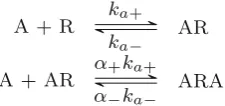
Fig. 1 Schematic representing the reactions resulting from the
binding of a single ligand A + R
ka+
ka− AR
A + AR α+ka+
α−ka− ARA
(B). Again, we relate to previous models and begin by finding the equilibrium solu-tion. This enables us to derive a condition for multiple inflections in the logDR curve for total bound ligand A, which this time depends on multiple mechanistic binding cooperativity coefficients and the concentration ofB. The ODE model for competition dynamics is linear as before, but its analytical solution is more laborious to compute. We again simulate the binding dynamics to explore the effects of the dynamic coopera-tivity factors. In Sect.4, we conclude with a discussion of our main results, underlining our contribution to the literature, and considering dynamic modelling in the context of mathematics supporting drug discovery.
2 Initial Model: Single Ligand
2.1 Model Formulation
In this initial model, we consider a single-ligand,A, binding to a pre-dimerised receptor complex. For the purposes of this paper, we assume all dimers are homodimers and so consist of two identical receptors bound together. We denote these dimers asRfor simplicity in the model but keep the assumption that ligand molecules can bind to either side of the dimer. Association and dissociation rates areka+andka−, respectively, and
we assume there is no bias to which protomer the ligand molecule binds to first. As the second ligand binding may be affected by one side of the dimer being already bound, we introduce α = α+/α− which represents the equilibrium binding cooperativity, that is the factor change in affinity for the dimer when it is already ligand bound. The valueα=1 represents neutral cooperativity, andα >1 andα <1 represent positive and negative cooperativity, respectively. Figure1 shows the system of biochemical reactions. Since Rrepresents a dimer,A Ris the complex created by a single-ligand molecule binding to a protomer andA R Ais a dual bound receptor.
2.2 Differential Equations
Applying the law of mass action, the binding kinetics are governed by the following system of ordinary differential equations (ODEs):
d[R]
dt =ka−[A R] −ka+[A][R], (1a)
d[A R]
[image:4.439.275.388.60.113.2]d[A R A]
dt =α+ka+[A][A R] −α−ka−[A R A], (1c)
Conservation of receptors in the system allows us to give the total concentration of dimerised receptors asDtot = [R]+[A R]+[A R A]. We use this to reduce the system to
two ODEs which, taking[A]as a constant, we write in the form ofddtX(t)=MX(t)+f: d
dt
[A R]
[A R A]
=
−(ka−+ka+[A] +α+ka+[A]) α−ka−−ka+[A]
α+ka+[A] −α−ka−
[A R]
[A R A]
+
ka+[A]Dt ot
0
, (2)
with initial conditions
[A R](0) [A R A](0)
=
0 0
. (3)
2.3 Equilibrium Analysis
In the spirit of classical receptor theory, we first investigate the equilibrium behaviour of the system, in particular the effect of the equilibrium cooperativity factorα. The equilibrium relationships are
[A R] =KA[A][R], (4a)
[A R A] =αKA[A][A R], (4b)
whereKA=ka+/ka−is the equilibrium association constant andα=α+/α−is the
equilibrium binding cooperativity. The total concentration of dimers is
Dtot= [R] + [A R] + [A R A]
= [R](1+KA[A] +αK2A[A]
2),
(5)
which we can combine with equations (4) to express the equilibrium concentrations in terms of parameters only, giving
[R] = 1
1+KA[A] +αK2A[A]2
Dtot, (6a)
[A R] = KA[A]
1+KA[A] +αK2A[A]2
Dtot, (6b)
[A R A] = αK
2
A[A]
2
1+KA[A] +αK2A[A]2
Dtot. (6c)
-12 -10 -8 -6 -4 -2 0 2 Log10[A]
0 0.5 1 1.5 2
Abound 10-10
-12 -10 -8 -6 -4 -2 0 2
Log10[A] 0
0.2 0.4 0.6 0.8 1
Rbound 10-10
+=1e-07 +=1e-03 +=1e-02 +=1e-01 += 1 += 10 += 100 += 1000
-12 -10 -8 -6 -4 -2 0 2
Log
10[A]
0 0.2 0.4 0.6 0.8 1
[AR]
10-10
-12 -10 -8 -6 -4 -2 0 2
Log
10[A]
0 0.2 0.4 0.6 0.8 1
[ARA]
10-10
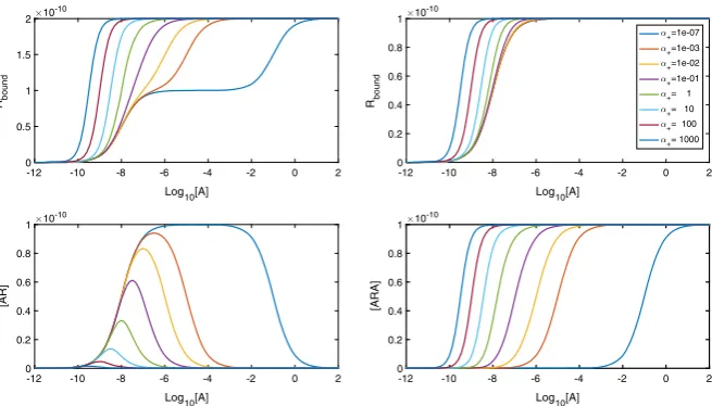
Fig. 2 LogDR curves forαranging from extreme negative to extreme positive cooperativity. Association
and dissociation rates are kept atka+=1×10⁷M−1s−1andka−=0.1 s−1, respectively, andDtotis set at 1×10⁻¹⁰M. We see that extra inflections appear inAboundwhen we have very negative cooperativity
interest, since this is often an experimentally measurable quantity (May et al.2011). At equilibrium, we have Abound = [A R] +2[A R A]due to a single-ligand molecule
being bound in[A R]and two-ligand molecules being bound in[A R A]. We therefore find
Abound= (
KA[A] +2αK2A[A]2)
1+KA[A] +αK2A[A]2
Dtot. (7)
This result is equivalent to the result (Giraldo2008) states when discussing a mecha-nistic model for a single-ligand binding to a dimerised receptor. As the maximal ligand bound is 2Dtot, we can calculate theEC50value forAbound(the concentration giving
half-maximal effect) as
A50=
1
KA√α.
(8)
Figure2shows how the equilibrium cooperativity factorαaffects the log dose– response (logDR) binding relationship. Increasing cooperativity leads to dimers becoming dual bound for lower concentrations of[A]and lower peaks in[A R].
Fur-ther, for Abound, biphasic logDR curves with multiple inflections are possible. With
extreme negative cooperativity, we see three inflections in the curve instead of just one. It can be shown (“Appendix B” ) that the inflection point that appears in all curves is at the point[A] =1/KA√α, which in this case is the same value as theEC50due to the
[image:6.439.57.385.55.242.2]Since the existence of extra inflections depends onαwe seek a condition onαfor when these appear. Following the calculation in “Appendix B,” we find that for three inflections we require
0< α <1/16. (9)
We note that this is different from Giraldo’s dimer cooperativity index condition for apparent cooperativity (Giraldo2008). From a curve-fitting perspective,α =1/4 is mechanistically negatively cooperative, but would give apparent cooperativity in the Hill function sense (see Giraldo2008). When (9) holds, the inflection at[A] = A50
changes from a rising inflection point to a falling one and we get two extra inflection points, one for[A]<A50and one for[A]>A50at the points
[A] = 1−8α±
√
(16α−1)(4α−1)
2αKA .
(10)
We see in Fig.2that this results in a biphasic curve. We note here that a biphasic logDR curve with three inflections as shown would not be seen for monomeric receptors. An experimental logDR curve may be suggestive of pre-dimerised receptors and very negative cooperativity.
2.4 Binding Dynamics–Analytical Solutions
The exact solution to the initial value problems2,3may be constructed by calculating the eigenvalues of the coefficient matrix and by using the method of undetermined coefficients (“Appendix D”), or by the method of Laplace transform (as in Motulsky and Mahan1984). Both methods give the analytical solutions as:
[A R](t)= ka+[A]Dtot
det(M)
λ2(α−ka−+λ1)eλ1t−λ1(α−ka−+λ2)eλ2t
λ1−λ2 +α−ka−
,
(11)
[A R A](t)= α+k
2
a+[A]2Dtot
det(M)(λ1−λ2)
λ2eλ1t−λ1eλ2t+λ1−λ2, (12)
where the eigenvalues of the coefficient matrixM are
λ1=
Tr(M)+Tr(M)2−4 det(M)
/2, (13a)
λ2=
Tr(M)−Tr(M)2−4 det(M)
/2, (13b)
and Tr(M)and det(M)are the trace and determinant ofM, respectively, given by:
Tr(M)= −(α−+1)ka−+(α++1)ka+[A]
<0, (14a)
=α−ka2−
1+KA[A] +αK2A[A]2
>0, (14b)
Our response of primary interest is the total concentration of ligand bound, Abound,
which is given by
Abound(t)=
ka+[A]Dtot det(M)
λ2(α−ka−+λ1+2α+ka+[A])eλ1t−λ1(α−ka−+λ2+2α+ka+[A])eλ2t+α−ka−+2α+ka+[A]
λ1−λ2
. (15)
The solution has two exponential components, meaning we would expect to see bi-exponential time courses in general. It can be shown (“Appendix C”) that not only are eigenvaluesλ1andλ2real and distinct but they are also always negative, since all parameters in the model are positive. Further,λ1gives the slow component of the dynamics, whileλ2gives the fast component. Clearly, ast → ∞, the exponential
components will decay to zero and we recover the equilibrium concentrations as
[A R] = α−ka+ka−[A]Dtot
det(M) , [A R A] =
α+k2
a+[A]2Dtot
det(M) , (16)
giving the total ligand bound at equilibrium as
Abound=
ka+[A]Dtot
det(M)
α−ka−+2α+ka+[A]
, (17)
equivalent to (6).
Having analytical solutions for the dynamics allows time courses to be plotted without the need for numerical ODE solvers. This is particularly useful for pharma-cologists without numerics expertise, allowing them to construct exact solutions for any parameter values in software packages such as Microsoft Excel or GraphPad Prism
(accepted). In this respect, the dynamics for our dimer binding model have the same
analytical structure as Motulsky–Mahan dynamics (Motulsky and Mahan1984). In “Appendix H,” we show a sample MATLAB code for construction of the analytical solution.
2.5 Results
Here we present numerical results which demonstrate the effects of cooperative dynam-ics across dimerised receptors. Figure3shows the binding of ligandAto the dimerised receptor [R] with the ligand being added as a constant quantity. Initially, ligand molecules bind singly to dimers, creating an increase in[A R]. As time increases, a
positive cooperativity factor means that the chance of a second ligand molecule bind-ing to the sbind-ingularly bound dimer is increased; thus,[A R A]increases. This increase
in[A R A]also has the effect of reducing[A R]which then falls towards zero. Hence,
0 10 20 30 40 50 60 70 80 90 100 t
0 0.5 1 1.5 2
Concentration
10-10
A
bound
[R] [AR] [ARA]
Fig. 3 The binding of ligandAto a pre-dimerised receptor results in a surge in[A R], while positive cooperativity leads to most dimers becoming dual bound. Parameter values are ka+=1×10⁷M−1s−1 andka−=0.1 s−1for association and dissociation rates while keeping[A]constant at 1×10⁻⁸M. Also
α+=2 andα−=0.01, giving positive cooperativity, and Dtot=1×10⁻¹⁰M
0 20 40 60 80 100
Time
0 0.5 1 1.5 2
Abound
10-10
[A]=1e-10 [A]=1e-09 [A]=1e-08 [A]=1e-07 [A]=1e-06 [A]=1e-05
0 20 40 60 80 100
Time
0 0.5 1 1.5 2
[AR]
10-11
0 20 40 60 80 100
Time
0 0.2 0.4 0.6 0.8 1
[ARA]
10-10
Fig. 4 Binding dynamics with varying[A]in the system. With high levels of[A], we no longer see peaks in[A R]. Here, ka+ = 1×10⁷M−1s−1andka− = 0.1 s−1, α+ =2 andα− = 0.01 with Dtot = 1×10⁻¹⁰M
to look at Fig.4. In this, we consider a range of values of[A]and study the effect this has on the binding dynamics. It is clear that not only doesAboundincrease to a higher
equilibrium concentration as[A]increases, but the equilibration timescale is shorter. For low[A],[A R]apparently approaches equilibrium monotonically, whereas a peak in[A R](t)occurs for high concentrations of A. The time at which a possible local extremum occurs is
t = −
log
α−ka−+λ1 α−ka−+λ2
λ1−λ2 . (18)
For a peak in[A R](t)(see “Appendix E”), we require
ka+[A]> α−ka−, (19)
[image:9.439.107.334.55.201.2] [image:9.439.55.386.260.350.2]0 20 40 60 80 100 Time
0 0.5 1 1.5 2
Abound
10-10
+=1e-04 +=1e-02 +=1e-01 += 1 += 10 += 1000
0 20 40 60 80 100 Time
0 1 2 3 4 5
[AR]
10-11
0 20 40 60 80 100 Time
0 0.2 0.4 0.6 0.8 1
[ARA]
10-10
Fig. 5 Binding dynamics with varyingα. As we move from positive to negative cooperativity, we see a
more pronounced peak in[A R]withAboundtending to lower concentrations. Here,ka+=1×10⁷M−1s−1 andka−=0.01 s−1,[A] =1×10⁻⁸M,Dtot=1×10⁻¹⁰M. We fixα−=1 so cooperativity varies viaα+
[A R]peak =
ka+[A]Dtot
det(M) ⎛
⎝−(α−ka−+λ1)
α−ka−+λ1
α−ka−+λ2
λ1
λ2−λ1
+α−ka−
⎞
⎠.
(20)
In Fig.5, we study the effect ofαonAbound(t). Clearly, the binding rate for a second ligand to the dimer increases and decreases for positive and negative cooperativity, respectively. We see a peak in[A R](t)whose timing and concentration are dependent onα+. Asα+increases, the peak in[A R]decreases and occurs earlier. Both[A R A]
andAboundincrease asα+increases.
3 Two-Ligand System
3.1 Model Formulation
We now introduce a second ligand,B, to the system. The rationale for this is that quan-tification of effects of unlabelled ligands can be achieved by competition experiments with labelled and unlabelled ligands, as seen in previous studies involving monomeric and dimeric receptors (Motulsky and Mahan1984; May et al.2011; Durroux2005; Franco et al.2006). The kinetics of this system are key in highlighting and quantifying allosteric interactions across dimerised receptors, as indicated by May et al. (2011), who discuss the influence of an unlabelled ligand on the dissociation (washout) kinetics of a labelled ligand, when dimers are present.
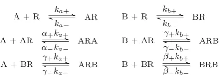
[image:10.439.54.385.51.146.2]A + R ka+
ka− AR B + R
kb+
kb− BR
A + AR α+ka+
α−ka− ARA B + AR
γ+kb+
γ−kb− ARB
A + BR γ+ka+
γ−ka− ARB B + BR
β+kb+
β−kb− BRB
Fig. 6 Schematic showing the binding possibilities with two ligands in the system
3.2 Differential Equations
As the total concentration of receptors is given by
Dtot= [R] + [A R] + [B R] + [A R A] + [A R B] + [B R B], (21)
we may eliminate[R]to give a system of five linear ODEs:
d[A R]
dt = −(ka+[A] +ka−+α+ka+[A] −γ+kb+[B])[A R] −ka+[A][B R]
+ (α−ka−−ka+[A])[A R A] +(γ−kb−−ka+[A])[A R B]
− ka+[A][B R B] +ka+[A]Dtot, (22a)
d[B R]
dt = −kb+[B][A R] −(kb+[B] +kb−+γ+kb+[A] +β+kb+[B])[B R]
− kb+[B][A R A] +(γ−kb−−kb+[B])[A R B]
+ (β−kb−−kb+[B])[B R B] +kb+[B]Dtot, (22b)
d[A R A]
dt =α+ka+[A][A R] −α−ka−[A R A], (22c)
d[A R B]
dt =γ+kb+[B][A R] +γ+ka+[A][B R]
− γ−kb−[A R B] −γ−ka−[A R B], (22d)
d[B R B]
dt =β+kb+[B][B R] −β−kb−[B R B]. (22e)
with initial conditions
⎛ ⎜ ⎜ ⎜ ⎜ ⎝
[A R](0) [B R](0) [A R A](0) [A R B](0) [B R B](0)
⎞ ⎟ ⎟ ⎟ ⎟
⎠=
⎛ ⎜ ⎜ ⎜ ⎜ ⎝
0 0 0 0 0
⎞ ⎟ ⎟ ⎟ ⎟
⎠. (23)
[image:11.439.106.334.52.134.2]3.3 Equilibrium Analysis
Once the system reaches equilibrium, we have the set of relations
[A R] =KA[A][R], [B R] =KB[B][R], (24a)
[A R A] =αK2A[A]2[R], [A R B] =γKAKB[A][B][R],
[B R B] =βK2B[B]2[R]. (24b)
The receptor conservation law therefore gives that
Dtot = [R](1+KA[A] +KB[B] +αK2A[A]2
+γKAKB[A][B] +βK2B[B]
2).
(25)
Here we consider, as in May et al. (2011), competition experiments where ligandAis labelled and ligandBis unlabelled. We can clearly see that, providing[B]is fixed,
[R],[A R],[B R],[A R B],[B R B] →0, and[A R A] →Dtotas[A] → ∞. (26)
The total concentration of bound ligand A(assumed an experimentally measurable quantity) is
Abound= [A R] +2[A R A] + [A R B], (27)
which, using Eqs. (24) and (25), gives
Abound=
KA[A] +2αK2A[A]2+γKAKB[A][B]
1+KA[A] +KB[B] +αK2A[A]2+γKAKB[A][B] +βKB2[B]2
Dtot.
(28)
As the maximalAboundfor varying[A]remains as 2Dtot, we calculate the EC50 for
Aboundas
A50 =
1
KA
1+KB[B] +βK2B[B]2
α , (29)
which we note is independent of the A-B cooperativity factorγ. In Figs.7,8,9, we show the effects of each of the cooperativity factorsα, β, γ in turn. In each case, we plot logDR curves forAboundfor a range of values for[B].
-15 -10 -5 0 5 Log 10[A] 0 0.5 1 1.5 2 Abound
10-10 =0.00001
[B]=1e-11 [B]=1e-10 [B]=1e-09 [B]=1e-08 [B]=1e-07 [B]=1e-06 [B]=1e-05
-15 -10 -5 0 5
Log 10[A] 0 0.5 1 1.5 2 Abound
10-10 =0.001
-15 -10 -5 0 5
Log 10[A] 0 0.5 1 1.5 2 Abound
10-10 =0.1
Fig. 7 LogDR curve for varyingα+shows extra inflections when we have low A-A cooperativity
regard-less of[B]. Plot parameters areka+ = kb+ = 1×10⁷M−1s−1,ka− = kb− = 0.1 s−1,[A] =
1×10⁻⁸M,Dtot=1×10⁻¹⁰M. All other cooperativity values are set to 1
-15 -10 -5 0 5
Log10[A] 0 0.5 1 1.5 2 Abound
10-10 =0.00001
[B]=1e-11 [B]=1e-10 [B]=1e-09 [B]=1e-08 [B]=1e-07 [B]=1e-06 [B]=1e-05
-15 -10 -5 0 5
Log10[A] 0 0.5 1 1.5 2 Abound
10-10 =0.001
-15 -10 -5 0 5
Log10[A] 0 0.5 1 1.5 2 Abound
10-10 =0.1
Fig. 8 LogDR curve for varyingβ+shows extra inflections appear when we have both low B-B
cooper-ativity and low[B]. Plot parameters areka+=kb+=1×10⁷M−1s−1,ka−=kb−=0.1 s−1,[A] =
1×10⁻⁸M,Dtot=1×10⁻¹⁰M. All other cooperativity values are set to 1
smallαrequires very large[A]to effect this downturn in[A R]and[A R B], giving
plateaus at the maximal response in the logDR for[A R]and[A R B]. It is these plateaus
that change the nature of the original inflection point for Abound, as well as creating
two extra inflections.
Figure8shows the effect of varying the B-B cooperativity factor,β. We see extra inflections appearing for conditions of both lowβand high[B]. For high[B]and small
β <1, a relatively large proportion of receptor will be in[B R]complexes, unless[A]
is sufficiently large. Again, corresponding logDR curves for[A R]and[A R B]exhibit local maxima (see Fig.10).
In Fig.9, we show the effects of A-B cooperativityγand see that, for extra inflec-tions,γ is required to be high as opposed to low. We again require there to be a high concentration ofBin the system. The individual species curves in Fig.11again show the requirement of sufficiently large[A]for a downturn in[A R]and[A R B], but this
time with the largest[A R B]values corresponding to largeγ.
Investigating these extra inflections inAbound(“Appendix G”), we find that there is
always an inflection point at
[A] = 1
KA
1+KB[B] +βKB2[B]2
[image:13.439.56.386.49.151.2] [image:13.439.54.388.205.301.2]-15 -10 -5 0 5 Log 10[A] 0 0.5 1 1.5 2 Abound
10-10 =10
[B]=1e-11 [B]=1e-10 [B]=1e-09 [B]=1e-08 [B]=1e-07 [B]=1e-06 [B]=1e-05
-15 -10 -5 0 5
Log 10[A] 0 0.5 1 1.5 2 Abound
10-10 =1000
-15 -10 -5 0 5
Log 10[A] 0 0.5 1 1.5 2 Abound
10-10 =100000
Fig. 9 LogDR curve for varyingγ+shows extra inflections when we have high A-B cooperativity as
well as low[B]. Plot parameters areka+ = kb+ = 1×10⁷M−1s−1,ka−= kb− =0.1 s−1,[A] =
1×10⁻⁸M,Dtot=1×10⁻¹⁰M. All other cooperativity values are set to 1
-14 -12 -10 -8 -6 -4 -2 Log10[A]
0 1 2 3 4 5 [R] 10-11 =1e-05 =1e-03 =1e-01 = 1 = 10 = 1000
-14 -12 -10 -8 -6 -4 -2 Log10[A]
0 0.5 1 1.5 2 2.5 [AR] 10-11
-14 -12 -10 -8 -6 -4 -2 Log10[A]
0 1 2 3 4 5 [BR] 10-11
-14 -12 -10 -8 -6 -4 -2 Log10[A]
0 0.2 0.4 0.6 0.8 1 [ARA] 10-10
-14 -12 -10 -8 -6 -4 -2 Log10[A]
0 0.5 1 1.5 2 2.5 [ARB] 10-11
-14 -12 -10 -8 -6 -4 -2 Log10[A]
[image:14.439.56.385.50.151.2]0 0.2 0.4 0.6 0.8 1 [BRB] 10-10
Fig. 10 Individual species plots for a varyingβ. Plots were created with parameters KA = KB =
108M−1, α=γ=1,[B] =10−5M,Dtot=10−10M
-14 -12 -10 -8 -6 -4 -2 Log10[A]
0 1 2 3 4 [R] 10-11 =1e-05 =1e-03 =1e-01 = 1 = 10 = 1000
-14 -12 -10 -8 -6 -4 -2 Log10[A]
0 0.5 1 1.5 2 2.5 [AR] 10-11
-14 -12 -10 -8 -6 -4 -2 Log10[A]
0 1 2 3 4 [BR] 10-11
-14 -12 -10 -8 -6 -4 -2 Log10[A]
0 0.2 0.4 0.6 0.8 1 [ARA] 10-10
-14 -12 -10 -8 -6 -4 -2 Log10[A]
0 0.2 0.4 0.6 0.8 1 [ARB] 10-10
-14 -12 -10 -8 -6 -4 -2 Log10[A]
0 1 2 3 4 [BRB] 10-11
Fig. 11 Individual species plots for a varyingγ. Plots were created with parametersKA = KB =
[image:14.439.52.387.199.369.2] [image:14.439.55.386.403.573.2]0 5 10 15 20 25 30 t
0 0.2 0.4 0.6 0.8 1
Concentration
10-10
[image:15.439.107.335.55.202.2][R] [AR] [BR] [ARA] [ARB] [BRB]
Fig. 12 In the time course plot, we see peaks in both[A R]and[B R]. Parameter values:ka+=kb+=
1×10⁷M−1s−1,ka− = kb− = 0.1 s−1, α+ = β+ = γ+ = 2, α− = β− = γ− = 0.01,[A] =
1×10⁻⁸M,[B] =2×10⁻⁸M,Dtot=1×10⁻¹⁰M
We further find that extra inflections appear under the condition
16α(1+KB[B] +βK2B[B]
2) < (γ
KB[B] +1)2. (31)
Again we have an extra inflection at either side of the original one, at the points
[A] = m
2−8αn±(m2−16αn)(m2−4αn)
2αKAm ,
(32)
wherem=1+γKB[B]andn=1+KB[B] +βKB2[B]2.
3.4 Time Course Results
Analytical solutions for the system (22) are theoretically possible, given that the system is linear. However, the task of computing eigenvalues exactly becomes laborious and impractical; we instead construct the solutions by numerical evaluation of the eigen-values. A numerical ODE solver could also be used. Here we present time course simulations for two-ligand competition.
In Fig.12, we show time courses for each receptor state, for conditions of positive A-A, A-B and B-B cooperativities. We note[A R]and[A R A]dynamics similar to the single-ligand problem. Initially, a single-ligand molecule binds to one of the free receptors in the dimer, increasing[A R]before the positive cooperativity factor soon after binds a second ligand molecule, thus increasing[A R A]and lowering[A R].
In Fig.13, we see the effectαhas on the time course dynamics of the system. We look at a range of values ofαwhile keepingβandγfixed, giving neutral cooperativity. It is clear that regardless of the A-A cooperativity, we get peaks in both[A R]and[B R].
0 10 20 30 t
0 0.5 1 1.5
Abound 10-10
=1e-07 =1e-02 =1e-01 = 1 = 10 = 1000
0 10 20 30
t 0
0.5 1 1.5
[AR]
10-11
0 10 20 30
t 0
0.5 1 1.5 2 2.5
[BR]
10-11
0 10 20 30
t 0
2 4 6 8
[ARA]
10-11
0 10 20 30
t 0
0.5 1 1.5 2 2.5
[ARB]
10-11
0 10 20 30
t 0
1 2 3 4
[BRB]
[image:16.439.54.385.52.242.2]10-11
Fig. 13 Asα+increases, the peak in[A R]decreases, while the peak in[B R]becomes more pronounced. Parameter values:ka+=kb+=1×10⁷M−1s−1,ka−=kb−=0.1 s−1,[A] =1×10⁻⁸M,[B] =
2×10⁻⁸M,Dtot=1×10⁻¹⁰M. All other cooperativity factors are set to 1
αincreases, we also see that[A R A]increases and both[A R B]and[B R B]decrease. Further, peaks are apparent in[A R B]and, for largeα, in[B R B].
In Fig.14, we vary cooperativity factorβ. Non-monotonic behaviour is clearly shown for all receptor states except [B R B], and the potential for non-monotonic
signalAbound is clearly demonstrated.
In Fig.15, we demonstrate the effect of varyingγ. As molecules ofAandBbecome bound to free receptors, we again see[A R]and[B R]increase. With smallγ, a second
Aor B molecule causes[A R A]and[B R B]to increase, while[A R B]remains low. Asγincreases past neutral cooperativity, we begin to see instead that it is the alternate ligand that binds to singularly bound receptors, meaning that[A R B]increases, while [A R A]and[B R B]remain low.
4 Discussion
0 10 20 30 t 0 2 4 6 8 Abound 10-11 =1e-07 =1e-02 =1e-01 = 1 = 10 = 1000
0 10 20 30
t 0 0.5 1 1.5 [AR] 10-11
0 10 20 30
t 0 1 2 3 4 [BR] 10-11
0 10 20 30
t 0 0.5 1 1.5 [ARA] 10-11
0 10 20 30
t 0 0.5 1 1.5 2 2.5 3 [ARB] 10-11
0 10 20 30
[image:17.439.56.386.51.245.2]t 0 0.2 0.4 0.6 0.8 1 [BRB] 10-10
Fig. 14 Asβincreases, the peak in[B R]decreases, while the peak in[A R]becomes more pronounced. Parameter values:ka+ = kb+ = 1×10⁷M−1s−1,ka− =kb− = 0.1 s−1,[A] =1×10⁻⁸,[B] =
2×10⁻⁸,Dtot=1×10⁻¹⁰M. All other cooperativity factors are set to 1 so cooperativity is neutral for A-A and A-B and B-B cooperativity depends solely onβ+
0 10 20 30
t 0 0.2 0.4 0.6 0.8 1 Abound 10-10 =1e-07 =1e-02 =1e-01 = 1 = 10 = 1000
0 10 20 30
t 0 0.5 1 1.5 2 [AR] 10-11
0 10 20 30
t 0 0.5 1 1.5 2 2.5 3 [BR] 10-11
0 10 20 30
t 0 0.5 1 1.5 [ARA] 10-11
0 10 20 30
t 0 0.2 0.4 0.6 0.8 1 [ARB] 10-10
0 10 20 30
t 0 1 2 3 4 5 [BRB] 10-11
Fig. 15 Asγ increases, the peak in both[A R]and[B R]decreases. Parameter values:ka+= kb+ =
1×10⁷M−1s−1,ka−=kb−=0.1 s−1,[A] =1×10⁻⁸M,[B] =2×10⁻⁸M,Dtot=1×10⁻¹⁰M. All other cooperativity factors are set to 1 so cooperativity is neutral for A-A and B-B and A-B cooperativity depends solely onγ+
Time course computation for our models is straightforward, given the analyt-ical solutions we have developed. However, there are interesting features in the equilibrium logDR curves for the experimental readout (signal)Abound. We have noted
[image:17.439.54.386.305.490.2]binding. Multiphasic features in logDR curves are not reproducible by standard Hill functions (Veroli et al.2015) which only support single inflection curves. For single-ligand binding, multiphasic logDR curves theoretically rule out monomeric receptor binding as the only ligand binding mechanism; such experimental data therefore would suggest another binding setup, possibly due to dimeric receptors. The existence of multiple inflections depends on the level ofcooperativityacross a dimerised receptor, and importantly we are able to give a condition on the single-ligand cooperativity factor for a three-inflection curve (9). The practical use of this condition is clearly in assessing the sign and magnitude of cooperativity towards quantitative classifica-tion of drug–receptor interacclassifica-tions. Given that Hill funcclassifica-tions are not suitable for fully characterising multiphasic logDR curves (Veroli et al.2015), our analysis here goes beyond dimer cooperativity indices which stem in part from cooperativity in the Hill function sense (Giraldo2008); the present work concernsmechanistic cooperativity
which is explicit in the original model schematic, as opposed to empirical measures from a more limited model. In Veroli et al. (2015), it is noted that multiphasic logDR curves have particular importance in a number of contexts including cancer phar-macology, and effort should be made to move beyond Hill function fitting wherever possible.
Two-ligand competition at GPCR homodimers has previously been discussed and modelled (May et al. 2011). In addition to the therapeutic relevance of agonist– antagonist competition (May et al. 2011; Bridge et al. 2010), for homodimeric receptors, dissociation kinetic assays may represent a more sensitive forum for detect-ing negative cooperativity than logDR analysis alone. As such, we have reduced the model of May et al. (2011) and outlined the analytical solution structure for the time-dependent problem. Further, considering a system with a labelled ligand
Aand an unlabelled ligand B, we are able to find conditions on[B]and the three cross-dimer cooperativity factors for multiple inflections in the logDR curve for
Abound (Eq. 31), which again is designed to aid interpretation of experimental data
and clear identification of parameter regimes which may have therapeutic signifi-cance.
Our simple models of ligands binding to constitutive homodimers, and particularly the explicit statement and elucidation of analytical results, represent an important addition to receptor theory. We remark that this should be considered only the foun-dation of the theory for binding and activation dynamics of GPCR dimers. There is a clear pathway for building on this foundation to expand upon this model towards simulating and understanding the potential diversity binding and signalling outcomes of non-monomeric receptors. In particular, the following natural extensions and con-siderations should be explored in future work.
1. Heterodimeric GPCRs are widely acknowledged to exist (Smith and Milligan
2. Higher-order complexes may exist (Smith and Milligan2010; Juška2008), and while a general functional signalling model for annth-order oligomer may be impractical, a ligand binding model of the type developed in the current work should be possible and may be valuable in distinguishing between orders of oligomer.
3. Here, we have assumed that all dimeric receptors are constitutively produced, are the only receptor entities and have not considered the dimerisation process itself. However, a mixture of monomers, dimers and higher oligomers may exist (Smith and Milligan2010; Milligan2004), and ligand-induced effects on the dimerisation process have also been noted for GPCRs (Smith and Milligan2010; Bai2004) and other receptors (Mac Gabhann and Popel2007). Therefore, we propose to expand the model to include constitutive and ligand-induced dimerisation dynamics. This will allow theoretical investigation of questions put forth in Milligan (2004) regard-ing the effects of fraction of receptors which are dimers, dynamics and lifetime of dimerisation and the effect of ligands. Further modelling in this direction will draw on dimerisation models (Vera et al.2008; Mac Gabhann and Popel2007), towards a general, hybrid model for constitutive and ligand-induced dimers and ligand binding. Further complexity may be possible within a dimer population, whereby only a fraction of dimers may support cross-dimer crosstalk (Durroux
2005).
4. In keeping with classical analytical pharmacology approaches, we have first con-sidered models for ligand binding; the cooperativity factorsα, β, γ arebinding
cooperativities. A diverse range of pharmacologicaleffectsis theoretically possible
from dimeric receptors, in terms of receptor activation and signalling dynam-ics (Milligan2004). Much is yet to be understood about signalling downstream of dimerised receptors, and how to distinguish between ligand–receptor level crosstalk and downstream crosstalk when interpreting experimental data (Milligan
2006, 2009; Chabre et al.2009). A natural extension of our model will include receptor activation (Giraldo2008), G protein binding (Milligan2009; Bai2004), and ultimately G protein activation and cycling (Woodroffe et al.2010; Bridge
2009). In moving towards simulating downstream functional effects, new mod-elling studies will require consideration of cross-dimer cooperativity in (i) ligand binding, (ii) receptor activation and (iii) G protein binding.
cooper-0 20 40 60 80 100 120 140 160 180 200 0
1 2 3 4 5 6x 10
−11
t Abound
[image:20.439.73.361.58.200.2]B=1e−06 B=1e−07 B=1e−08 B=1e−09 B=0
Fig. 16 Binding then washout experiments, for labelled ligandAand unlabelled ligandB, varying[B]. Firstly binding ofAin the absence ofB, then dissociation ofA, withAbeing washed out, with varying concentrations of B. The dissociation curves depend on[B], indicating cooperativity across the dimer (such a result would not be seen for monomeric receptor). Parameter values:ka+ =1×10⁷M−1s−1,
ka− = 0.03 s−1,[A] =3×10⁻⁹M,kb+ =1×10⁷M−1s−1,kb− =0.01 s−1, α+= 0.005, α− = 1, β+=1, β−=10, γ+=1, γ−=10. All three equilibrium cooperativities are negative, in qualitative agreement with (May et al.2011)
ativities are reported rather than all individual kinetic constants. The analysis in May et al. (2011) further suggests that a combination of association and washout experiments will be useful in estimating kinetic parameters relating to dimerised receptor binding. The simplified models presented in the current work will be used to simulate such experiments, and a detailed SIA will be performed towards param-eterising ligand–dimer interactions. In Fig.16, we show an initial simulation of binding followed by washout, in qualitative agreement with the results presented in May et al. (2011).
The current work provides a theoretical foundation for the study of ligands bind-ing dimerised receptors. We consider this theory as a vital step towards the potential exploitation of dimerised receptors in a therapeutic and drug discovery context. Under-standing the functional, physiological and therapeutic significance of receptor dimers is an ongoing challenge (Smith and Milligan2010), with some questions still out-standing over the possible requirement of dimerisation for receptor function (Milligan
Acknowledgements CW is supported by a Swansea University/College of Science PhD studentship. We acknowledge helpful discussions with Professor Venkat Kanamarlapudi and Dr. Vivi Rottschäfer.
Open Access This article is distributed under the terms of the Creative Commons Attribution 4.0 Interna-tional License (http://creativecommons.org/licenses/by/4.0/), which permits unrestricted use, distribution, and reproduction in any medium, provided you give appropriate credit to the original author(s) and the source, provide a link to the Creative Commons license, and indicate if changes were made.
A Simplification of the May et al. Model
System (22) is seen to be a simplification of the model developed by May et al. (2011), equivalent by taking
ka+=
ka+
2 , ka−=ka− kb+=
kb+
2 , kb−=kb−, (33)
α+=2α+, α−=α−
2 , β+=2β+,
β−=β−
2 , γ+=2γ+, γ−=
γ−
2 , (34)
noting that
[A R] = [A R]
2 , [B R] = [B R]
2 , [A R B] =
[A R B]
2 , (35)
where a tilde denotes a parameter or variable in the May et al. (2011) model.
B Extra Inflections in the Single-Ligand
A
boundCurve
In Fig.2, we saw extra inflections in the logDR curve forAbound. We investigate these
and derive the condition given in Eq. (9). Writing Aboundin terms ofX=KA[A]for
simplification, we have
Abound =
X+2αX2
1+X+αX2Dtot. (36)
To investigate the inflections, we require d2Abound
dY2 where
Y =log10[A] =
lnKX A
ln 10 , (37)
(andX =KA10Y). Using Di Bruno’s Johnson (2002) formula for the chain rule for
second derivatives, we find
d2Abound
dY2 =
dX
dY
2
.d2Abound
dX2 +
d2X
dY2.
dAbound
Calculating each term individually, we have
dX
dY =KA10
Y
ln 10=Xln 10, (39)
d2X
dY2 =KA10
Y(
ln 10)2=X(ln 10)2, (40)
dAbound
dX =
1+4αX+αX2
(1+X+αX2)2Dtot, (41)
d2Abound
dX2 =
−2(1−2α+3αX+6α2X2+α2X3)
(1+X+αX2)3 Dtot. (42)
Substituting into (38), and after some simplification, we find
d2Abound
dY2 =
X(ln 10)2(1+(8α−1)X+(α−8α2)X3−α2X4)
(1+X+αX2)3 Dtot. (43)
To locate the possible inflection points, we find zeros ofd2Abound/dY2, which occur
when
X(1+(8α−1)X+(α−8α2)X3−α2X4)=0,
⇒ −X(αX2−1)(1−X+8αX+αX2)=0. (44) This gives the trivial solution atX =0 and solutions at
X = ±√1
α. (45)
However, we are only interested in positive solutions, so we conclude that we always have an inflection point atX =1/√α, that is when[A] =1/KA
√
α. We note that this is the same concentration of[A]that gives half the maximal response. Other possible inflections occur for rootsX >0 of the quadratic equation
1−X+8αX+αX2=0, (46)
which gives solutions at
X±= 1−8α±
(8α−1)2−4α
2α
= 1−8α± √
(16α−1)(4α−1)
2α . (47)
We see that we get a repeated root if
that is whenα=1/16 orα=1/4. However, we see that the root is only positive for
α=1/16. To get real and distinct solutions, we require
(16α−1)(4α−1) >0, (49)
that is whenα > 14 or whenα < 161. We also need to confirm whether the roots are positive or negative under these conditions. So first noting that
(1−8α)2−4α >0, (50)
⇒(1−8α)2>4α, (51)
⇒(1−8α)2−4α <8α−1. (52)
Now ifα < 1/16, then 1−8α > 1−1/2 =1/2 >0; thus, we have two positive roots under this condition. However, ifα >1/4, then 1−8α < 1−2 = −1 <0; hence, under this condition we get two negative roots. So we conclude that we get two possible extra inflection points under the condition 0< α <1/16.
To confirm that these are inflection points and classify the type of inflection, we consider d3Abound/dY3. Using the Di Bruno formula (see Johnson (2002)) for higher derivatives, or MATLAB’s Symbolic Toolbox, we find:
d3Abound
dY3 =
X(ln 10)3
1+(16α−4)X+(1−13α)X2+(8α−64α2)X3
+(α−13α2)X4+(16α3−4α2)X5+α3X6
(1+X+αX2)4 Dtot.
(53)
For theEC50value, atX =1/√α, and substituting this into the third derivative. After
some simplification, we have
−(ln 10)3(8α−2 √
α)
(2√α+1)2 Dtot, (54)
which we can see is positive for any 0< α <1/16 and negative for anyα >1/16. Similarly for the extra inflections, we found atX=τ1andX =τ2whenα <1/16. Substituting both of these in results in a value of
(ln 10)3(16α−1)
8(4α−1)2 Dtot, (55)
which clearly gives a negative result for any 0< α <1/16.
C Confirming the Eigenvalues of the Coefficient Matrix are Real,
Distinct and Negative
Before we can solve the system of equations to give analytical solutions, we need to know whether the eigenvalues, given in Eq. (13), of the coefficient matrixM are real and distinct so we can determine the form of the general solution. Being able to state whether these are also positive or negative allows us to analyse these solutions. The eigenvalues are defined as
λ1,2=
Tr(M)±Tr(M)2−4 det(M)
2
= Tr(M)±
Tr(M)2−4 det(M)
2 , (56)
so we can see that the discriminant is
D=Tr(M)2−4 det(M). (57)
ExpandingD, we have
D=Tr(M)2−4 det(M),
=(α−−1)2ka2−−2(α−−1)(α++1)ka+ka−[A]
+(α++1)2k2a+[A]2−4α+ka2+[A]2+4α+α−ka+ka−[A],
=(α−−1)2ka2−−2(α+α−+α−−α+−1)ka+ka−[A]
+(α++1)2k2a+[A]2−4α+ka2+[A]2+4α+α−ka+ka−[A],
=(α−−1)2ka2−−2(α+α−+α−−α+−1)ka+ka−[A]
+(α+−1)2k2a+[A]2+4α+α−ka+ka−[A],
=(α−−1)2ka2−+2(α+α−−α−+α++1)ka+ka−[A]
+(α+−1)2k2a+[A]2,
=(α−−1)2ka2−+2((α−−1)(α+−1)+2α+)ka+ka−[A]
+(α+−1)2k2a+[A]2,
=(α−−1)ka−+(α+−1)ka+[A]
2
+4α+ka+ka−[A],
>0. (58)
Hence,Dis always positive, providing that all parameters are positive.
We can also show that bothλ1andλ2are always negative. First noting that Tr(M)
is negative due to all terms being negative, and
⇒Tr(M)2>4 det(M) (60)
⇒Tr(M)2−4 det(M) <Tr(M). (61)
Thus, it is clear that both Tr(M) +Tr(M)2−4 det(M) < 0 and Tr(M)−
Tr(M)2−4 det(M) <0; hence, both eigenvalues are negative.
D Analytical Solutions for the Single-Ligand Dynamics
One of the main motivations for this paper is to be able to give exact solutions to the system, allowing for simulations to be run easily; hence, in this appendix we derive these solutions as stated in Eqs. (11) and (12). To find a solution to the system, we first find the eigenvalues of the coefficient matrix,M.
λ1,2=
Tr(M)±Tr(M)2−4 det(M)
2 . (62)
The eigenvectors corresponding to eigenvaluesλ1andλ2are
v1=
λ1+α−ka−
α+ka+[A]
, v2=
λ2+α−ka−
α+ka+[A]
. (63)
Thus, we can state that a solution to the system will be of the form
X(t)=c1v1eλ1t+c2v2eλ2t+Xp(t), (64)
whereXp(t)is a particular solution, found by solvingMX+f=0, thus
Xp=ka+[A]Dtot
det(M)
α−ka−
α+ka+[A]
. (65)
Ast → ∞, all other terms in the solution tend to zero, due toλ1,2always being
nega-tive; thus, the particular solution tells us what[A R]and[A R A]will be at equilibrium. We now use the initial conditions to solve the system and find the coefficientsc1and
c2, as
C=
c1
c2
= ka+[A]Dtot
det(M)(λ1−λ2)
λ2
−λ1
. (66)
[A R](t)= ka+[A]Dtot
det(M)
λ2(α−ka−+λ1)eλ1t−λ1(α−ka−+λ2)eλ2t
λ1−λ2 +α−ka−
,
(67)
[A R A](t)= α+k
2
a+[A]2Dtot
det(M)(λ1−λ2)
λ2eλ1t−λ1eλ2t+λ1−λ2. (68)
E A Condition for Existence of a Peak in
[
AR
]
(
t
)
As we saw in Figs.3,4, we sometimes get a peak in[A R](t). In this appendix, we investigate these peaks to find a condition Eq. (19) for peak existence and calculate this peak concentration Eq. (20) is. The peak time is given by Eq. (18)
t= −
ln
α−ka−+λ1 α−ka−+λ2
λ1−λ2 . (69)
For peak existence, we therefore require
α−ka−+λ1
α−ka−+λ2 >
0, (70)
whereλ2< λ1<0. Hence, we require, for a positive peak time,
0<α−ka−+λ1
α−ka−+λ2 <
1,
which requires that
α−ka−+λ1<0.
Sinceλ1=−(α−+1)ka−−(α++1)ka+[A]+√D
2 , whereDis the discriminant for the
coeffi-cient matrix, we find our requirement to be
0< (α++1)ka+[A] −(α−+1)ka−<
√
D,
which eventually gives
α−<KA[A]. (71)
To evaluate the peak concentration[A R], we take Eq. (18)
t = −
log
α−ka−+λ1 α−ka−+λ2
λ1−λ2 . (72)
ka+[A]Dtot det(M)
⎛ ⎜ ⎜ ⎝
λ2(α−ka−+λ1)
α−ka−+λ1
α−ka−+λ2
λ1
λ2−λ1 −λ
1(α−ka−+λ2)
α−ka−+λ1
α−ka−+λ2
λ2
λ2−λ1
λ1−λ2 +α−
ka−
⎞ ⎟ ⎟ ⎠
(73)
=ka+[A]Dtot det(M)
⎛ ⎜ ⎜ ⎝
λ2(α−ka−+λ1)−
α −ka−+λ1
α−ka−+λ2
λ1(α−ka−+λ2) αα−−kkaa−−++λλ12
λ1
λ2−λ1
λ1−λ2 +α−
ka−
⎞ ⎟ ⎟ ⎠
(74)
=ka+[A]Dtot det(M)
⎛ ⎜ ⎜ ⎝
(λ2(α−ka−+λ1)−λ1(α−ka−+λ1))
α−ka−+λ1
α−ka−+λ2
λ1
λ2−λ1
λ1−λ2 +α−
ka−
⎞ ⎟ ⎟
⎠ (75)
=ka+[A]Dtot det(M)
⎛ ⎜ ⎜ ⎝
(λ2−λ1)(α−ka−+λ1)
α −ka−+λ1
α−ka−+λ2
λ1
λ2−λ1
λ1−λ2 +α−
ka−
⎞ ⎟ ⎟
⎠ (76)
=ka+[A]Dtot det(M)
⎛
⎝−(α−ka−+λ1)
α−ka−+λ1 α−ka−+λ2
λ1
λ2−λ1
+α−ka− ⎞
⎠ (77)
as the corresponding concentration of[A R].
F Individual Species Dose–Response Curves
To further help us understand the behaviour observed in the logDR curves forAbound,
we look to the individual species plots. In Fig.17, we see plateaus in the logDR curves
of[A R]and[A R A]when we have very low A-A cooperativity. These are the main
contributions to the inflections in Abound.
-12 -10 -8 -6 -4 -2 0 Log10[A]
0 1 2 3 4 [R] 10-11 =1e-05 =1e-03 =1e-01 = 1 = 10 = 1000
-12 -10 -8 -6 -4 -2 0 Log10[A]
0 1 2 3 4 5 [AR] 10-11
-12 -10 -8 -6 -4 -2 0 Log10[A]
0 1 2 3 4 [BR] 10-11
-12 -10 -8 -6 -4 -2 0 Log 10[A] 0 0.2 0.4 0.6 0.8 1 [ARA] 10-10
-12 -10 -8 -6 -4 -2 0 Log 10[A] 0 1 2 3 4 5 [ARB] 10-11
[image:27.439.55.388.409.579.2]-12 -10 -8 -6 -4 -2 0 Log 10[A] 0 1 2 3 4 [BRB] 10-11
Fig. 17 Individual species plots for a varyingα. Plots were created with parametersKA =KB =1×
G Investigating the Extra Inflections in the Two-Ligand
A
boundcurve
Similarly to the single-ligand system, we also get extra inflections in theAboundcurve
when we have two ligands in the system. In this appendix, we investigate these to derive the condition given in Eq. (31) under which we get these extra inflections. We begin by writingAboundas
Abound =
X+2αX2+γX Y
1+X+Y +αX2+γX Y+βY2Dtot, (78)
where X = KA[A] andY = KB[B]. For possible inflections, we first calculate
d2Abound/d Z2where Z =log10[A] =ln(KXA)/ln 10. We find d2Abound
dZ2
=
X(ln 10)2((βY2+Y+1−αX2)
((α+αγY2)X2+(8α(βY2+Y+1)−(1+γY)2)X+(1+γY)(βY2+Y+1))
(1+X+Y+αX2+γX Y+βY2)3
(79)
= X(ln 10)2(n−α(X2)(mn+(8αn−m2)X+αm X2)
n+m X+αX2)3 (80)
wherem=1+γY andn=1+Y +βY2. Clearly, we have the trivial root atX =0 as well as a root when
n−αX2=0, (81)
that is when
X = ±
n
α. (82)
As we are only interested in positive roots, we conclude that we have a possible inflection at
Xc=
n
α, (83)
which corresponds to theEC50concentration. We also get extra roots when
mn+(8αn−m2)X+αm X2=0, (84)
which using the quadratic formula gives us
X±=m
2−8αn±(8α−m2)2−4αm2n
=m2−8αn±
(m2−16αn)(m2−4αn)
2αm . (86)
We see that we get a single, real root when
(m2−16αn)(m2−4αn)=0, (87)
that is whenm2 = 16αn or m2 = 4αn. However, we see that ifm2 = 4αn, then
X = −2n/m, hence a negative root. Whereas ifm2 =16αn, then X =4n/m, so we have a positive root. Thus, we can conclude that we have a possible inflection at
X =4n/munder the condition ofm2=16αn. Finally, we have two real distinct roots when
(m2−16αn)(m2−4αn) >0. (88)
Asm2−16αn <m2−4αn, then this holds if eitherm2 >16αn orm2<4αn. To confirm whether these conditions give positive or negative roots, we first note that
(m2−8αn)2−4αm2n >0 (89) ⇒(m2−8αn)2>4αm2n (90) ⇒(m2−8αn)2−4αm2n <m2−
8αn. (91)
Using this, we can state that ifm2>16αn, thenm2−8αn>16αn−8αn=8αn >0; hence, we have two positive roots. Conversely, if m2 < 4αn, then m2 −8αn <
4αn−8αn = −4αn < 0; hence, both roots are negative. Thus, we can conclude that we get two positive roots, and possible inflection points, under the condition
m2>16αn. That is
(1+γY)2>16α(1+Y +βY2). (92)
To confirm that these are in fact inflection points, we first confirm thatX−<Xc<
X+. First noting thatm2−16αn<m2−4αn ⇒(m2−16αn)2< (m2−16αn)(m2−
4αn)⇒m2−16αn<(m2−16αn)(m2−4αn), then we can state that
X−= m
2−8αn−(m2−16αn)(m2−4αn)
2αm (93)
< m2−8αn−(m2−16αn)
2αm (94)
= 8αn
2αm (95)
= 4n
=
16n2
m2 (97)
<
n
α =Xc. (98)
Thus, we can confirm thatX−<Xc. Also
X+= m
2−8αn+(m2−16αn)(m2−4αn)
2αm (99)
> m2−8αn
2αm (100)
=
(m2−8αn)2
4α2m2 (101)
>
4αm2n
4α2m2 (102)
=
n
α =Xc, (103)
hence confirming thatXc <X+. We now use the second derivative to confirm there is a
sign change at each of the points. We can see asX →0+, we haved2Abound/d Z2>0.
TakingXˆ−=4n/mas a point betweenX−andXc, we evaluate
d2Abound
dZ2
X= ˆX−
= −12n3(m2−16αn)2
m4 <0; (104)
thus, we can confirm there is an inflection point atX−with the curve changing from convex to concave. Taking Xˆ+=(m2−8αn)/2αmas a point betweenXcandX+,
we evaluate
d2Abound
dZ2
X= ˆX−
=(m2−8αn)((m2−8αn)2−4αm2n)2
32α3m4 >0; (105)
hence, there is a sign change at the pointXcwith the curve changing from convex to
![Fig. 3 The binding of ligandcooperativity leads to most dimers becoming dual bound. Parameter values are A to a pre-dimerised receptor results in a surge in [AR], while positive ka+ = 1 × 10⁷ M−1 s−1and ka− = 0.1 s−1 for association and dissociation rates](https://thumb-us.123doks.com/thumbv2/123dok_us/585523.558297/9.439.55.386.260.350/ligandcooperativity-parameter-dimerised-receptor-results-positive-association-dissociation.webp)
![Fig. 5 Binding dynamics with varyingmore pronounced peak in α. As we move from positive to negative cooperativity, we see a [AR] with Abound tending to lower concentrations](https://thumb-us.123doks.com/thumbv2/123dok_us/585523.558297/10.439.54.385.51.146/binding-dynamics-varyingmore-pronounced-positive-negative-cooperativity-concentrations.webp)
![Fig. 8 LogDR curve for varying β+ shows extra inflections appear when we have both low B-B cooper-ativity and low [B]](https://thumb-us.123doks.com/thumbv2/123dok_us/585523.558297/13.439.56.386.49.151/logdr-curve-varying-shows-inections-appear-cooper-ativity.webp)
![Fig. 9 LogDR curve for varying γ+ shows extra inflections when we have high A-B cooperativity aswell as low [B]](https://thumb-us.123doks.com/thumbv2/123dok_us/585523.558297/14.439.55.386.403.573/logdr-curve-varying-shows-extra-inections-cooperativity-aswell.webp)
![Fig. 12 In the time course plot, we see peaks in both [AR] and [BR]. Parameter values: ka+ = kb+ =1 × 10⁷ M−1 s−1, ka− = kb− = 0.1 s−1, α+ = β+ = γ+ = 2, α− = β− = γ− = 0.01, [A] =1 × 10⁻⁸ M, [B] = 2 × 10⁻⁸ M, Dtot = 1 × 10⁻¹⁰ M](https://thumb-us.123doks.com/thumbv2/123dok_us/585523.558297/15.439.107.335.55.202/fig-time-course-plot-peaks-parameter-values-dtot.webp)
![Fig. 13 As α+ increases, the peak in [AR] decreases, while the peak in [BR] becomes more pronounced.Parameter values: ka+ = kb+ = 1 × 10⁷ M−1 s−1, ka− = kb− = 0.1 s−1, [A] = 1 × 10⁻⁸ M, [B] =2 × 10⁻⁸ M, Dtot = 1 × 10⁻¹⁰ M](https://thumb-us.123doks.com/thumbv2/123dok_us/585523.558297/16.439.54.385.52.242/fig-increases-peak-decreases-pronounced-parameter-values-dtot.webp)
![Fig. 14 AsA-A and A-B and B-B cooperativity depends solely on β increases, the peak in [BR] decreases, while the peak in [AR] becomes more pronounced.Parameter values: ka+ = kb+ = 1 × 10⁷ M−1 s−1, ka− = kb− = 0.1 s−1, [A] = 1 × 10⁻⁸, [B] =2 × 10⁻⁸, Dtot =](https://thumb-us.123doks.com/thumbv2/123dok_us/585523.558297/17.439.54.386.305.490/cooperativity-depends-solely-increases-decreases-pronounced-parameter-values.webp)
