Computing motion in the primate's visual system

COMPUTING MOTION IN THE PRIMATE'S VISUAL SYSTEM

BY CHRISTOF KOCH

Computation and Neural Systems Program, Divisions of Biology and Engineering and Applied Sciences, 216-76, California Institute of Technology,

Pasadena, CA 91125, USA

H. TAICHI WANG and BIMAL MATHUR

Science Center, Rockwell International, Thousand Oaks, CA 91360, USA

Summary

Computing motion on the basis of the time-varying image intensity is a difficult problem for both artificial and biological vision systems. We will show how one well-known gradient-based computer algorithm for estimating visual motion can be implemented within the primate's visual system. This relaxation algorithm computes the optical flow field by minimizing a variational functional of a form commonly encountered in early vision, and is performed in two steps. In the first stage, local motion is computed, while in the second stage spatial integration occurs. Neurons in the second stage represent the optical flow field via a population-coding scheme, such that the vector sum of all neurons at each location codes for the direction and magnitude of the velocity at that location. The resulting network maps onto the magnocellular pathway of the primate visual system, in particular onto cells in the primary visual cortex (VI) as well as onto cells in the middle temporal area (MT). Our algorithm mimics a number of psychophysical phenomena and illusions (perception of coherent plaids, motion capture, motion coherence) as well as electrophysiological recordings. Thus, a single unifying principle 'the final optical flow should be as smooth as possible' (except at isolated motion discontinuities) explains a large number of phenomena and links single-cell behavior with perception and computational theory.

Introduction

One prominent school of thought holds that information-processing systems, whether biological or man-made, should follow essentially similar computational strategies when solving complex perceptual problems, in spite of their vastly different hardware (Marr, 1982). However, it is not apparent how algorithms developed for machine vision or robotics can be mapped in a plausible manner onto nervous structures, given their known anatomical and physiological con-straints. In this chapter, we show how one well-known computer algorithm for estimating visual motion can be implemented within the early visual system of primates.

performed in different ways in different biological systems. In the primate visual system, motion appears to be measured on the basis of two different systems, termed range and long-range processes (Braddick, 1974, 1980). The short-range process analyzes continuous motion, or motion presented discretely but with small spatial and temporal displacement from one moment to the next (apparent motion; in the human fovea both presentations must be within 15min of arc and with 60-100ms of each other). The long-range system processes larger spatial displacements and temporal intervals. A second, conceptually more important, distinction is that the short-range process uses the image intensity, or some filtered version of image intensity (e.g. filtered via a Laplacian-of-Gaussian or a difference-of-Gaussian operator), to compute motion, while the long-range process uses more high-level 'token-like' motion primitives, such as lines, corners, triangles etc. (Ullman, 1981). Among short-range motion processes, the two most popular classes of algorithms are the gradient method on the one hand (Limb & Murphy, 1975; Fennema & Thompson, 1979; Marr & Ullman, 1981; Hildreth, 1984; Yuille & Grzywacz, 1988) and the correlation, second-order or spatio-temporal energy methods on the other hand (Hassenstein & Reichardt, 1956; Poggio & Reichardt, 1973; van Santen & Sperling, 1984; Adelson & Bergen, 1985; Watson & Ahumada, 1985). Gradient methods exploit the relationship between the spatial and the temporal intensity gradient at a given point to estimate local motion, while the second class of algorithms multiplies a filtered version of the image intensity with a slightly delayed version of the filtered intensity from a neighboring point (a mathematical operation similar to correlation; hence their name (for a review, see Hildreth & Koch, 1987).

Computational theory

The problem in computing the optical flow field consists of labeling every point in a visual image with a vector, indicating at what speed and in what direction this point moves (for reviews on motion see Ullman, 1981; Nakayama, 1985; Horn, 1986; Hildreth & Koch, 1987). One limiting factor in any system's ability to accomplish this is the fact that the optical flow, computed from the changing image brightness, can differ from the underlying two-dimensional velocity field. This vector field, a purely geometrical concept, is obtained by projecting the three-dimensional velocity field associated with moving objects onto the two-dimen-sional image plane. A perfectly featureless rotating sphere will not induce any optical flow field, even though the underlying velocity field differs from zero almost everywhere. Conversely, if the sphere does not rotate but a light source, such as the sun, moves across the scene the computed optical flow will be different from zero even though the velocity field is not (Horn, 1986). In general, if the objects in the scene are strongly textured, the optical flow field should be a good approximation to the underlying velocity field (Verri & Poggio, 1987).

falling onto a retina or a phototransistor array is that the total derivative of the image intensity between two image frames separated by the interval dr is zero:

dl(x,y,t)/dt = 0. In other words, the image intensity seen from the point-of-view of

an observer located in the image plane and moving with the image, does not change. This conservation law is strictly only satisfied for translation of a rigid Lambertian body in planes parallel to the image plan (for a detailed error analysis see Kearney et al. 1987). This law will be violated to some extent for other types of movements, such as motion in depth or rotation around an axis. The question is to what extent this rule will be violated and whether the system built using this hypothesis will suffer from a severe 'visual illusion'.

Using the chain rule of differentiation, dl/dt = 0 can be reformulated as

Ixx+Iyy+I[ = VI- V+It = 0, where x' = dx/dt and y = dy/dt are the x and y

components of velocity V, and Ix = 91/dx, Iy = 31/dy and /, = 91/dt are the spatial

and temporal image gradients which can be measured from the image (vectors are printed in boldface). Formulating the problem in this manner leads to a single equation in two unknowns x',y. Measuring at n different locations does not help in general, since we are then faced with n linear equations in In unknowns. This type of problem is termed ill-posed (Hadamard, 1923). One way to make these problems well-behaved in a precise, mathematical sense, is to impose additional constraints in order to be able to compute unambiguously the optical flow field. The fact that we are unable to measure both components of the velocity vector is also known as the 'aperture' problem. Any system with a finite viewing aperture and the rule dl/dt = 0 can only measure the component of motion - 7 , / | V/| along the spatial gradient V7 = (Ix,Iy). The motion component perpendicular to the local

gradient remains invisible. In addition to the aperture problem, the initial motion data is usually noisy and may be sparse. That is, at those locations where the local visual contrast is weak or zero, no initial optical flow data exist (the featureless rotating sphere would be perceived as stationary), thereby complicating the task of recovering the optical flow field in a robust manner.

To solve this problem Horn & Schunck (1981) first introduced a 'smoothness constraint'. The underlying rationale for this constraint is that nearby points on moving objects tend to have similar three-dimensional velocities; thus, the projected velocity field should reflect this fact. Their algorithm finds the optical flow field which is as compatible as possible with the measured motion com-ponents, and also varies smoothly everywhere in the image. This flow field is determined by minimizing a cost functional L:

an ideal world free of noise, dl/dt should be zero; we here impose the condition that it should be as small as possible to account for unavoidable noise in the motion measurement stage. The terms in the second bracket represent a measure of the smoothness of the flow field, the parameter A controlling the compromise between the smoothness of the desired solution and its closeness to the data. The contribution of this term to L will be zero for a spatially constant flow field -induced by rigid motion in the plane — since all spatial derivatives will be zero. The smoothness constraint also stabilizes the solution against the unavoidable noise in the intensity measurements.

Since L is quadratic in x and y and therefore has a unique minimum, the final solution minimizing L will represent a trade-off between faithfulness in the data and smoothness, depending on a parameter A. The Horn & Schunck (1981) algorithm derives motion at every point in the image by taking into account motion in the surrounding area. It can be shown that it finds the qualitatively correct optical flow field for real images (for a mathematical analysis in terms of the theory of dynamic systems see Verri & Poggio, 1987). Such as area-based optical flow method is in marked contrast to the edge-based algorithm of Hildreth (1984); she proposes to solve the aperture problem by computing the optical flow along edges (in her case zero-crossings of the filtered image) using a variational functional very similar to that of equation 1.

The use of general constraints (as compared to very specific constraints of the type 'a red blob at desk-top height is a telephone', popular in early computer vision algorithms) is very common to solve the ill-posed problems of early vision (Poggio et al. 1985). Thus, continuity and uniqueness are exploited in the Marr & Poggio (1977) cooperative stereo algorithm, smoothness is used in surface interpolation (Grimson, 1981) and rigidity is used for reconstructing a three-dimensional figure from motion (structure-from-motion; Ullman, 1979).

Before we continue, it is important to emphasize that the optical flow is computed in two, conceptually separate, stages. In the first stage, an initial estimate of the local motion, based on spatial and temporal image intensities, is computed. Horn & Schunck's method of doing this (using dl/dt = 0) belongs to a broad class of motion algorithms, collectively known as gradient algorithms (Limb & Murphy, 1975; Fermema & Thompson, 1979; Marr & Ullman, 1981; Hildreth, 1984; Yuille & Grzywacz, 1988). A new variant of the gradient method, using

dVl/dt = 0 to compute local motion, leads to uniqueness of the optical flow, since

this constraint is equivalent to two linear independent (in general) equations in two unknowns (Uras et al. 1988). Thus, in this formulation, computing optical flow is not an ill-posed but an ill-conditioned problem. Alternatively, a correlation or second-order model could be used at this stage for estimating local motion (Hassenstein & Reichardt, 1956; Poggio & Reichardt, 1973; van Santen & Sperling, 1984; Adelson & Bergen, 1985; Watson & Ahumada, 1985; Reichardt et

al. 1988). However, for both principal (e.g. non-uniqueness of initial motion

However, while the optical flow generally varies smoothly from location to location, it can change quite abruptly across discontinuities. Thus, the flow field associated with a flying bird varies smoothly across the animal but drops to zero 'outside' the bird (since the background is stationary). In these cases of motion discontinuities usually encountered when objects move across each other -smoothing should be prevented (see below and Hutchinson et al. 1988).

The cost functional used to compute motion (equation 1) is a quadratic variational functional of a type common in early vision (Poggio et al. 1985), and can be solved using simple electrical networks (Poggio & Koch, 1985). The key idea is that the power dissipated in a linear electrical network is quadratic in the currents or voltages; thus, if the values of the resistances are chosen appropriately, the functional L to be minimized corresponds to power dissipation and the steady-state voltage distribution in the network corresponds to the minimum of L in equation 1. Data are introduced by injecting currents into the nodes of the network. Once the network settles into its steady state - dictated by Kirchhoff s & Ohm's laws - the solution can simply be read off by measuring the voltages at every node. Efforts are now under way (see, in particular, Luo et al. 1988) to build such resistive networks for various early vision algorithms in the form of miniaturized circuits using analog, subthreshold CMOS VLSI technology of the type pioneered by Mead (1989).

Implementation in a neuronal network

We will now describe a possible neuronal implementation of this computer vision algorithm. Specifically, we wih1 show that a reformulated variational functional equivalent to equation 1 can be evaluated within the known anatomical and physiological constraints of the primate visual system and that this formalism can explain a number of psychophysical and physiological phenomena.

Neurons in the visual cortex of mammals represent the direction of motion in a very different manner from resistive networks, using many neurons per location such that each neuron codes for motion in one particular direction (Fig. 1). In this representation, the velocity vector V(i,j) [where (/',/) are the image plane coordinates of the center of the cell's receptive field] is not coded explicitly but is computed across a population of n such cells, each of which codes for motion in a different direction (given by the unit vector ©k), such that:

v(i,j) = I v(t,j,k)e

. (2)

A k+l kk-l k' + l k' k'-l

9

S, T

y

9

-\

y

U, E

Transient channel

Reunal images

Sustained channel

Area VI

Direction-selective cells U

AreaMT

Optical flow

Orientation-selective cells E

Fig. 1. Computing motion in neuronal networks. (A) Simple scheme of our model. The image / is projected onto the rectangular 64 by 64 retina and sent to the first processing stage via the 5 and T channels. Subsequently, a set of n = 16 ON-OFF orientation- and direction-selective (U) cells code local motion in n different directions. Neurons with overlapping receptive field positions ij but different preferred directions 8k (indicated by arrows in the upper right-hand side of each

plane) are arranged here in n parallel planes. The ON subfield of one such U cell is shown in Fig. 8A. The output of both E and U cells is relayed to a second set of 64 by 64

V cells where the final optical flow is computed. The final optical flow is represented in

this stage, on the basis of a population coding V(l j ) = Z£_1 V(ij,k)Sv, with n = 16.

Each cell V(ij,k) in this second stage receives input from cells E and U at location ij as well as from neighboring V neurons at different spatial locations. (B) Block model of a possible neuronal implementation. The T and 5 streams originate in the retina and enter the primary visual cortex in layer 4C<* and 4C£. The output of VI projects from layer 4B to the middle temporal area (MT). We assume that the ON-OFF orientation-and direction-selective neurons E orientation-and U are located in VI, orientation-and the final optical flow is assumed to be represented by the V units in area MT.

inhibitory inputs exceed the excitatory ones, the neuron is silent. We then require at least n = 4 neurons to represent all possible directions of movement. Note that in this representation the individual components V(i,j,k) are not the projections of the velocity field V(i j ) onto the direction ©k (except for n = 4).

Let us now consider a two-stage model for extracting the optical flow field based on cortical physiology (Fig. 1). Following Marr & Ullman (1981), we assume that in a pre-processing stage the intensity distribution /(/,/) is projected onto the image plane and relayed to the first cortical processing stage via two sets of cells:

(i,j) (3)

and

n i J > , ( )

at

where G is the two-dimensional Gaussian filter (with a2 = 4 pixels; Marr & Hildreth, 1980; Marr & Ullman, 1981). The V2G filter is very similar to the difference-of-Gaussian or Mexican hat-shaped receptive fields of retinal ganglion cells (Enroth-Cugell & Robson, 1966). This stage then models the filtering performed by retinal ganglion cells. S and T cells, however, only represent a first-order approximation of the visual transformations occurring in the retina and the lateral geniculate nucleus, because retinal ganglion cells always show some transient behavior - different from equation 3 - and do not respond instan-taneously, as would be expected from equation 4. However, little would be gained at this early stage in our understanding of cortical processing by using much more sophisticated cellular models (for such a detailed dynamic description of cat retinal X cells see Victor, 1987).

In the first processing stage, the local motion information (the velocity component along the local spatial gradient) is measured using n ON-OFF orientation- and direction-selective cells U{i,j,k), each with preferred direction indicated by the unit vector 0k (here the V neurons and the U neurons have the

same number of directions and the same preferred directions for the sake of simplicity, even though it is not necessary):

™*-

(5)

where e is a constant and V^ the spatial derivative along the direction 0k. This

each with preferred axis given byQk(ke {l...n}) exist. The cell U{i,j,k) responds

optimally if a bar or grating oriented at right angles to Ok moves in direction Gk.

Our definition of U differs from the standard gradient model U = — T/VkS, by

including a gain control term, e, such that t/does not diverge if the visual contrast of the stimulus decreases to zero; thus, U-* — TVkS as | V^^S| —>• 0. Under these

conditions of small stimulus contrast, our model can be considered a second-order model, similar to the correlation or spatio-temporal energy models (Hassenstein & Reichardt, 1956; Poggio & Reichardt, 1973; Adelson & Bergen, 1985) and the output of the U cell is proportional to the product of a transient cell (T) and a sustained simple cell with an odd-symmetric receptive field (VkS); thus, the

response of U is proportional to the magnitude of velocity. For large values of stimulus contrast, i.e. \VkS\ > e, U-* — T/VkS. Thus, our model of local motion

detection appears to contain aspects of both gradient and second-order methods, depending on the exact experimental conditions (for a further discussion of this issue, see Koch etal. 1989).

Finally, as an input to our second stage, we also require a set of ON-OFF, orientation-selective but not direction-selective neurons:

) \ . (6)

The absolute value operation (| • |) ensures that these neurons only respond to the amplitude of the spatial gradient, but not to its sign.

We have now progressed from registering and convolving the image in the retina to computing and representing local motion information within the first stage of our network. In the second processing stage, we determine the final optical flow field by computing the activity of a second set of cells, V. The state of these neurons - coding for the final (global) optical flow field - is evaluated by minimizing a reformulated version of the functional in equation 1. The first term expresses the fact that the final velocity field should be compatible with the initial data, i.e. with the local velocity component measured along the spatial gradient ('velocity constraint line'). In other words, the velocity at location (i,j), V(i,j) = 22 = i V(i,j,k)&k should be compatible with the local motion term U:

U= I [ I V(iJ,k') cos (*' -k)- U(iJ,k) V ET(iJ,k), (7)

where cos (k'—k) represents the cosine of the angle between 0k' and 0k, and E(i,j,k) is the output of an orientation-selective neuron raised to the mth power.

This term ensures that the local motion components U(i,j,k) only have an influence when there is an appropriately oriented local pattern; in other words, E™ prevents velocity terms incompatible with the measured data from contributing significantly to Lo. Thus, we require that the neurons E(i,j,k) do not respond

significantly to directions differing from Ok. If they do, L$ will increasingly contain

approximately 60°), m = 2 gave satisfactory responses. Equation 7 directly corresponds to the first term in the variational functional of Horn & Schunck (1981), equation 1.

The second, smoothing, term in equation 1 can be reformulated in a straightfor-ward manner by replacing the partial derivatives of x and y by their components in terms of V(i,j,k) [for instance, the x component of the vector V(i,j) is given by Z* V(i,j,k)cosSk]. This leads to:

x cos(A:' - k)V{i,j,k'). (8)

We are now searching for the neuronal activity level V(i,j,k) that minimizes the functional LQ + kL\. Similar to the original Horn & Schunck's functional, equation 1, the reformulated variational functional is quadratic in V(i,j,k), so we can find this state by evolving V(i,j,k) on the basis of the steepest descent rule:

aV(ij,k)_ djLp + XLr) k)

The contribution from the Lo term to the right-hand side of this equation has the

form:

cos(k-k')E

(i,j,k') \U(i,j,k')- £ cos(k'- k")V(i,j,k") , (10)

,j,k")] ,

J

while the contribution from the Lj term has the form:

A I cos(fc - k')[V(i - l,j,k') + V(i + l,j,k') + V(i,j - 1,/c') + V(iJ

k'

,k')} . (11)

The terms in equations 10 and 11 are all linear in either UOT V. This enables us to view them as the linear synaptic contributions of the U and V neurons towards the activity of neuron V(iJ,k). The left-hand term of equation 9 can be interpreted as a capacitative term, governing the dynamics of our model neurons. In other words, in evaluating the new activity state of neuron V{i,j,k), we evaluate equations 10 and 11 by summing all the contributions from V and U of the same location i,j as well as neighbouring V neurons and subsequently using a simple numerical integration routine to compute the new state at time t+At. The appropriate network carrying out these operations is shown schematically in Fig. 1A.

Correspondence to cortical anatomy and physiology

The neuronal network we propose to compute optical flow (Fig. 1) maps directly onto the primate visual system. Two major visual pathways, the parvo-and the magnocellular, originate in the retina parvo-and are perpetuated into higher visual cortical areas. Magnocellular cells appear to be the ones specialized to process motion information (for reviews, see Livingstone & Hubel, 1988; DeYoe & van Essen, 1988), since they respond faster and more transiently and are more sensitive to low-contrast stimuli than parvocellular cells. Parvocellular neurons, in contrast, are selective for form and color.

We do not identify our S and T channels with either the parvo- or the magno-pathway since this is not crucial to our model. Furthermore, reversibly blocking either the magno- or the parvocellular input to cells in the primary cortex leads to a degradation but not to the abolition of orientation- and direction-selectivity (Malpelli et al. 1981). Different from our model, cortical cells therefore appear to compute the local estimate of motion in either of the two pathways. Our current model does require that one set of cells signals edge information while a second population is sensitive to temporal changes in intensity (motion or flicker). We approximate the spatial receptive field of our retinal neurons using the Laplacian-of-Gaussian operator and the temporal properties of our transient pathway by the first derivative. Thus, the response of our U neurons increases linearly with increasing velocity of the stimulus. This is, of course, an oversimplification and more realistic filter functions should be used (see above).

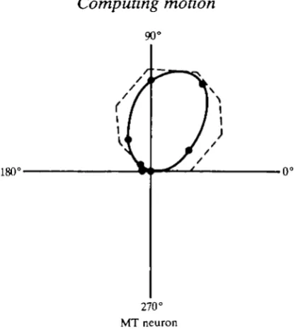
Both the parvo- and the magnocellular pathways project into layer 4C of the primary visual cortex. Here the two pathways diverge, magnocellular neurons projecting to layer 4B (Lund et al. 1976). Cells in this layer are orientation- as well as direction-selective (Dow, 1974). Layer 4B cells project heavily to a small but well-defined visual area in the superior temporal sulcus called the middle temporal area (MT; Allman & Kass, 1971; Baker et al. 1981; Maunsell & van Essen, 1983a). All cells in MT are direction-selective and tuned for the speed of the stimulus; the majority of cells are also orientation-selective. Moreover, irreversible chemical lesions in MT cause striking elevations in psychophysically measured motion thresholds, but have no effect on contrast thresholds (Newsome & Pare, 1988). These findings all support the thesis that area MT is at least partially responsible for mediating motion perception. We assume that the orientation- and direction-selective E and U cells corresponding to the first stage of our motion algorithms are located in layers 4B or 4C in the primary visual cortex or possibly in the input layers of area MT, while the V cells are located in the deeper layers of area MT. Inspection of the tuning curve of a V model cell in response to a moving bar reveals its similarity with the superimposed experimentally measured tuning curve of a typical MT cell of the owl monkey (Fig. 2).

180°

270° MT neuron

Fig. 2. Polar plot of the median neuron (solid line) in the medial temporal cortex (MT) of the owl monkey in response to a field of random dots moving in different directions (Baker et al. 1981). The tuning curve of one of our model V cells in response to a moving bar is superimposed (dashed line). The distance from the center of the plot is the average response in spikes per second. Both the cell and its model counterpart are direction-selective, since motion towards the upper right quadrant evokes a maximal response whereas motion towards the lower left quadrant evokes no response. Figure courtesy of J. Allman and S. Petersen.

well as from MT neurons V at the same location i,j but with differently oriented receptive fields k'. No spatial convergence or divergence occurs between our U and V modules, although this could be included. The first part of equation 10 gives the synaptic strength of the Uto V projection [cos{k-k')Em{i,j,k')U{i,j,k')\. if the

preferred direction of motion of the presynaptic input U(i,j,k') differs by no more than ±90° from the preferred direction of the postsynaptic neuron V(i,j,k), the

U—> V projection will depolarize the postsynaptic membrane. Otherwise, it will

act in a hyperpolarizing manner, since the cos(k—k') term will be negative. Notice that our theory predicts neurons from all cortical orientation columns k' (which could be located in either VI or in the superficial layers of MT) projecting onto the

Vcells, a proposal which could be addressed using anatomical labeling techniques.

The synaptic interaction contains a multiplicative nonlinearity (U-E7"). This veto term can be implemented using a number of different biophysical mechan-isms, for instance 'silent' or 'shunting' inhibition (Koch etal. 1982). The smoothness term Lx results in synaptic connections among the V neurons, both

connections acts in either a de- or a hyperpolarizing manner, depending on the sign of cos(k—k') as well as on their relative locations (see equation 11).

We will next discuss an elegant psychophysical experiment, strongly supporting a two-stage model of motion computation (Adelson & Movshon, 1982; Welch, 1989). Moreover, since MT cells in primates, but not cells in VI, appear to mimic the behavioral response of humans to the psychophysical stimulus, such exper-iments can be used as probes to dissect the different stages in the processing of perceptual information.

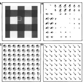
If two identical sine or square gratings are moved at an angle past each other, human observers perceive the resulting pattern as a coherent plaid, moving in a direction different from the motion of the two individual gratings. The direction of the resultant plaid pattern ('pattern velocity') is given by the 'velocity space combination rule' and can be computed from knowledge of the local 'component velocities' of the two gratings (Adelson & Movshon, 1982; Hildreth, 1984). One such experiment is illustrated in Fig. 3. A vertical square grating is moved horizontally at right angles over a second horizontal square grating of the same contrast and moving at the same speed vertically. The resulting plaid pattern is seen to move coherently to the lower right-hand corner (Adelson & Movshon, 1982), as does the output of our algorithm. Note that the smoothest optical flow field compatible with the two local motion components (one from each grating) is identical to the solution of the velocity space combination rule. In fact, for rigid planar motion, as occurs in these experiments, this rule as well as the smoothness constraint lead to identical solutions, even when the velocities of the gratings differ (illustrated in Fig. 4A,B). Notice that the velocity of the coherent pattern is not simply the vector sum of the component velocity (which would predict motion towards the lower right-hand corner in the case illustrated in Fig. 4A,B).

If the contrast of both gratings is different, the component velocities are weighted according to their relative contrast. As long as the contrasts of the two gratings differ by no more than approximately one order of magnitude, observers still report coherent motion, but with the final pattern velocity biased towards the direction of motion of the grating with the higher contrast (Stone et al. 1988). Since our model incoporates such a contrast-dependent weighting factor (in the form of equation 5), it qualitatively agrees with the psychophysical data (Fig. 4C,D).

Movshon et al. (1985) repeated Adelson & Movshon's plaid experiments while recording from neurons in the striate and extrastriate macaque cortex (see also Albright, 1984). All neurons in VI and about 60 % of cells in MT only responded to the motion of the two individual gratings (component selectivity; Movshon et al. 1985), similar to our U(i,j,k) cell population, while about 30 % of all recorded MT cells responded to the motion of the coherently moving plaid pattern (pattern selectivity), mimicking human perception. As illustrated in Fig. 3, our V cells behave in this manner and can be identified with this subpopulation.

V

fr

t

4

\

\

N

N*

N*

N*

\

\

N*

N.

s*

\

\

\

s*

s*

\

\

\

\

s.

\

\

\

\

\

\

\

\

\

\

\

\

\

\

\

\

\

\

\

\

\

\

\

\

\

\

\

\

\

\

Fig. 3. Mimicking perception and single-cell behavior. (A) Two superimposed square gratings, oriented orthogonal to each other, and moving at the same speed in the direction perpendicular to their orientation. The amplitude of the composite is the sum of the amplitude of the individual bars. (B) Response of a patch of 8 by 8 direction-selective simple cells U (outlined in A) to this stimulus. The outputs of all n = 16 cells are plotted in a radial coordinate system at each location as long as the response is significantly different from zero; the lengths are proportional to the magnitudes. (C) The output of the V cells using the same needle diagram representation after 2-5 time constants. (D) The resulting optical flow field, extracted from C via population coding, corresponding to a plaid moving coherently towards the lower right-hand corner, is similar to the perception of human observers (Adelson & Movshon, 1982) as well as to the response of a subset of MT neurons in the macaque (Movshon et al. 1985).

128

B

>. N* Nl N» ^i > >i

SWWNS

^ ^ ^ ^ ^ ^ ^ N, N. N,

N N N, N.

N N

N ,

s,

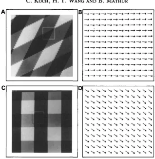
Fig. 4. Additional coherent plaid experiments. (A) Two gratings moving towards the lower right (one at —26° and one at —64°), the first moving at twice the speed of the second. The final optical flow, coded via the V cells, of a 12 by 12 pixel patch (outlined in A) is shown in B, corresponding to a coherent plaid moving horizontally towards the right. The final optical flow is within 5% of the correct flow field. (C) Similar to the experiment illustrated in Fig. 3, except that the contrast of the horizontally oriented grating only has 75 % of the contrast of the vertically oriented gTating. The final optical flow (D) is biased towards the direction of motion of the vertical grating, in agreement with psychophysical experiments (Stone etal. 1988; compare with Fig. 3D).

cells should respond to an extended bar (or grating) moving parallel to its edge. Even though, in this case, no motion information is available if only the classical receptive field of the MT cell is considered, motion information from the trailing and leading edges will propagate along the entire bar. Thus, neurons whose receptive fields are located away from the edges will eventually (i.e. after several tens of milliseconds) signal motion in the correct direction, even though the direction of motion is parallel to the local orientation. This neurophysiological prediction is illustrated in Fig. 8A,B.

B

Fig. 5. Figure-ground response. (A) The first frame of two random-dot stimuli. The area outlined was moved 1 pixel to the left. (B) The final population-coded velocity field, signals the presence of a blob, moving towards the left. The outline of the displaced area is superimposed onto the final optical flow.

containing no edges or intensity discontinuities. Our algorithm responds well to random-dot motion, as long as the spatial displacement between two consecutive frames is not too large (Fig. 5).

130

B

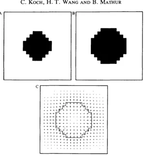
Fig. 6. Motion in depth. (A,B) Two images, featuring an approaching circular structure, expanding by 1 pixel in every direction. (C) Even though this type of motion violates the constraint underlying our algorithm, the network finds the qualitatively correct solution.

Psychophysics

We now consider the response of the model to a number of stimuli which generate strong psychophysical percepts. We have already discussed the plaid experiments (previous section), in which our smoothness constraint leads to the correct, perceived interpretation of coherent motion.

Fig. 7. Psychophysical illusions. In motion coherence, random dot figures (A) are shown. However, all dots have a common motion component; in this case, all dots move 1 pixel towards the top, but have a random horizontal displacement component (±2, ±1 and Opixels). (B) The final velocity field only shows the motion component common to all dots. Humans observe the same phenomena (Williams & Sekuler, 1984). (C) In motion capture, the motion of a low-spatial-frequency grating super-imposed onto a random-dot display 'captures' the motion of the random dots. (D) The entire display seems to move towards the right. Human observers suffer from the same optical illusion (Ramachandran & Anstis, 1983a).

frequency grating - is illustrated in Fig. 7C,D. However, in order to explain the non-intuitive finding that the capture effect becomes weaker for high-frequency gratings, a version of our algorithm which works at multiple spatial scales is required.

1984) can be accounted for using a specific smoothness constraint. Our algorithm also reproduces this visual illusion quite well (Fig. 7A,B)- In fact, it is surprising how often the Gestalt psychologists use the words 'smooth' and 'simple' when describing the perceptual organization of objects (for instance in the formulation of the key law of Pragnanz; Kofka, 1935; Kohler, 1969). Thus, one could argue that these psychologists intuitively captured some of the constraints used in today's computer vision algorithms.

Smoothing, that is that the flow field at one location influences motion at a different location, will not occur instantaneously. The differential equation implemented by our network (equations 9-11) can be considered to be a spatial discretized version of a parabolic differential equation, a family of partial differential equations whose members include the diffusion and the heat equation. We thus expect the time it takes to travel a certain distance to be proportional to the square of this distance. There exists some psychophysical support for this notion. Neighboring flashed dots can impair the speed discrimination of a pair of briefly flashed dots in an apparent motion experiment (Bowne & McKee, 1989). This 'motion interference' is time-selective, such that the optimal time of occurrence for the stimuli to interfere with the task increases with increasing distance between the two.

Our algorithm is able to mimic another illusion of the Gestalt psychologists: y motion (Lindemann, 1922; Kofka, 1931). A figure which is exposed for a short time appears with a motion of expansion and disappears with a motion of contraction, independent of the sign of contrast. Our algorithm responds in a similar manner to a flashed disk (Wang etal. 1989). A similar phenomenon has previously been reported for both fly and man (Blilthoff & Gotz, 1979). This illusion arises from the initial velocity measurement stage and does not rely on the smoothness constraint.

Our model so far does not take into account temporal integration of velocity information over more than two frames [all simulations were always carried out with only two frames: I{x,y,t) and I(x,y,t + At)]. This is an obvious oversimplifica-tion. From careful psychophysical measurements we know that optimal velocity discrimination requires about 80-100 ms (McKee & Welch, 1985). Furthermore, a number of experiments argue for a 'temporal recruitment' (P. J. Snowden & O. J. Braddick, personal communication) or 'motion inertia' (Ramachandran & Anstis, 1983ft) effect, such that the previously perceived velocity or direction of velocity influences the currently perceived velocity. Such a phenomenon could be reproduced by including into the variational functional of equation 1 a term which smooths over time, such as dV/dl.

Motion transparency

experiment (Fig. 3) differ by an order of magnitude in visual contrast, i.e. one grating having a strong and the other a weak contrast, or if the two gratings differ significantly in spatial frequency, they tend not to be perceived as moving coherently. Perceptually, observers report seeing two gratings sliding past or over each other. The significant fact is that in these cases, more than one unique velocity is associated with a location in visual space.

Welch & Bourne (1989) propose that motion transparency could be decided at the level of the striate cortex by neurons that compare the local contrast and temporal frequency content of the moving stimuli. If either of these two quantities differ substantially - probably caused by two distinct objects - a decision not to cohere would be made. We could then assume within our framework that this decision - occurring somewhere prior to our smoothing stage - prevents smoothing from occurring by blocking the appropriate connections among the V cells with spatially distinct receptive fields. This could be accomplished by setting the synaptic connection strength to zero either via conventional synaptic inhibition or via the release of a neurotransmitter or neuropeptide acting over relatively large cortical areas. The notion that motion transparency prevents smoothing among the V cells presupposes that the perceptual apparatus now has access to the individual motion components V(i,j,k), instead of to the vector sum V(i,j) of equation 2; only this assumption can explain the perception of two or more velocity vectors at any one location. Simple electrophysiological experiments could provide proof for or against our conjecture. For instance, it would be very intriguing to know how the pattern-selective cells of Movshon et al. (1985) in area MT respond to the two moving gratings of Adelson & Movshon (1982; see Figs 3 and 4). We know that if the gratings cohere, the cells respond to the motion of the plaid. How would these cells respond, however, if the two gratings do not cohere and motion transparency is perceived by the human observer?

Motion discontinuities

The major drawback of this and all other motion algorithms is the degree of smoothness required, smearing out any discontinuities in the flow field, such as those arising along occluding objects or along a figure-ground boundary. A powerful idea to deal with this problem was proposed by Geman & Geman (1984; see also Blake & Zisserman, 1987), who introduced the concept of binary line processes which explicitly code for the presence of discontinuities. We adopted the same approach for discontinuities in the optical flow by introducing binary horizontal (lh) and vertical (/*") line processes representing discontinuities in the

Geman, 1984). In our deterministic approximation to their stochastic search technique, a modified version of the variational functional in equation 1 must be minimized (Hutchinson et al. 1988). This functional is, different from before, non-quadratic or non-convex, that is it can have many local minima. Domain-independent constraints about motion discontinuities, such as that they occur in general along extended contours and that they usually coincide with intensity discontinuities (edges), are incorporated into this approach (Geman & Geman, 1984; Poggio et al. 1988). As before, some of these constraints may be violated under laboratory conditions (such as when a homogeneous black figure moves over an equally homogeneous black background and the motion discontinuities between the figure and the ground do not coincide with the edges, since there are no edges) and the algorithm computes an optical flow field different from the underlying two-dimensional velocity field (in this case, the computed optical flow field is zero everywhere). However, for most natural scenes, these motion discontinuities lead to a dramatically improved performance of the motion algorithm (see Hutchinson et al. 1988).

We have not yet implemented motion discontinuities into the neuronal model. It is known, however, that the visual system uses motion to segment different parts of the scene. Several authors have studied the conditions under which disconti-nuities (in either speed or direction) in motion fields can be detected (Baker & Braddick, 1982; van Doom & Koenderink, 1983; Hildreth, 1984). Van Doom & Koenderink (1983) concluded that perception of motion boundaries requires that the magnitude of the velocity difference be larger than some critical value, a finding in agreement with the notion of processes that explicitly code for motion boundaries. Recently, Nakayama & Silverman (1988) studied the spatial interac-tion of mointerac-tion among moving and stainterac-tionary waveforms. A number of their results could be re-interpreted in terms of our motion discontinuities.

f t 4

—

•

• • - . . . ' <

• • • f

. . . , .

' f

• • • « . f . I » 1—. ,. .

• • . <.

S * ' « * • • • • • «

t < «. *

• • • • » • * • • • r

u

Fig. 8. Robustness of the neuronal network. A dark bar (outlined in all images) is moved parallel to its orientation towards the right. (A) Owing to the aperture problem, those U neurons whose receptive field only 'see' the straight elongated edges of the bar - and not a corner - will fail to respond to this moving stimulus, since it remains invisible on the basis of purely local information. The ON subfield of the receptive field of a vertically oriented U cell is superimposed for comparison. (B) It is only after information has been integrated, following the smoothing process inherent in the second stage of our algorithm, that the V neurons respond to this motion. Type II cells of Albright (1984) in MT should respond to this stimulus whereas cells in VI do not. (C) Subsequently, we randomly 'lesion' 25 % of all V neurons, that is, their output is always set to 0. The resulting distribution of V cells is obviously perturbed. (D) However, given the redundancy build into the V cells (at each location n = 16 neurons signal the direction of motion), the final population-coded velocity field only differs on average by 3 % from the flow field computed with no 'damaged' neurons.

Conclusion

in the face of hardware errors such as missing connections (Fig. 8). While the details of our algorithm are bound to be incorrect, it does explain qualitatively a number of perceptual phenomena and illusions, as well as electrophysiological experiments, on the basis of a single unifying principle: the final optical flow should be as smooth as possible. We are much less satisfied with our formulation of the initial, local stage of motion computation, because the detailed properties of direction-selective cortical cells in cat and primates do not agree with those of our U cells. The challenge here is to bring the biophysics of such motion-detecting cell into agreement with the well-explored phenomenological theories of psychophy-sics and computational vision (Grzywacz & Koch, 1988; Suarez & Koch, 1989).

The performance of our motion algorithm implemented via resistive grids (Hutchinson et al. 1988) is substantially improved following the introduction of processes which explicitly label for the existence of motion discontinuities, across which no smoothing should occur. It would be surprising if the nervous system has not made use of such an idea.

References

ADELSON, E. H. & BERGEN, J. R. (1985). Spatio-temporal energy models for the perception of motion. /. opt. Soc. Am. A 2, 284-299.

ADELSON, E. H. & MOVSHON, J. A. (1982). Phenomenal coherence of moving visual patterns. Nature, Lond. 200, 523-525.

ALBRIGHT, T. L. (1984). Direction and orientation selectivity of neurons in visual are a MT of the macaque. J. Neurophysiol. 52, 1106-1130.

ALLMAN, J. M. &KASS, J. H. (1971). Representation of the visual field in the caudal third of the middle temporal gyms of the owl monkey (Aotus trivirgatus). Brain Res. 31, 85-105.

ALLMAN, J., MIEZIN, F. & MCGUINNESS, E. (1985). Direction- and velocity-specific responses from beyond the classical receptive field in the middle temporal area (MT). Perception 14, 105-126.

BAKER, C. L. & BRADDICK, O. J. (1982). Does segregation of differently moving areas depend on relative or absolute displacement. Vision Res. 7, 851-856.

BAKER, J. F., PETERSEN, S. E., NEWSOME, W. T. & ALLMAN, J. M. (1981). Visual response properties of neurons in four extrastriate visual areas of the owl monkey (Aotus trivirgatus): a quantitative comparison of medial, dorsomedial, dorsolateral and middle temporal areas. J. Neurophysiol. 45, 397-416.

BLAKE, A. & ZISSERMAN, A. (1987). Visual Reconstruction. Cambridge, MA: MTT Press.

BOWNE, S. F. & MCKEE, S. P. (1989). Motion interference in speed discrimination. J. opt. Soc. Am. A (in press).

BOLTHOFF, H. H. & GOTZ, K. G. (1979). Analogous motion illusion in man and fly. Nature, Lond. 278, 636-638.

BOLTHOFF, H. H., LITTLE, J. J. & POGGIO, T. (1989). Parallel computation of motion: computation, psychophysics and physiology. Nature, Lond. (in press).

BRADDICK, O. J. (1974). A short-range process in apparent motion. Vision Res. 14, 519-527.

BRADDICK, O. J. (1980). Low-level and high-level processes in apparent motion. Phil. Trans. R. Soc. Ser. B 290, 137-151.

CYNADER, M. & REGAN, D. (1982). Neurons in cat visual cortex tuned to the direction of motion in depth: effect of positional disparity. Vision Res. 22, 967-982.

DEYOE, E. A. & VAN ESSEN, D. C. (1988). Concurrent processing streams in monkey visual cortex. Trends Neurosci. 11, 219-226.

ENROTH-CUGELL, C. & ROBSON, J. G. (1966). The contrast sensitivity of retinal ganglion cells of the cat. /. Physiol, Lond. 187, 517-552.

FENNEMA, C. L. & THOMPSON, W. B. (1979). Velocity determination in scenes containing several moving objects. Comput. Graph. Image Proc. 9, 301-315.

GEMAN, S. & GEMAN, D. (1984). Stochastic relaxation, Gibbs distribution and the Bayesian restoration of images. IEEE Trans. Pattern anal. Machine Intell. 6, 721-741.

GRIMSON, W. E. L. (1981). From Images to Surfaces. Cambridge, MA: MIT Press.

GRZVWACZ, N. M. & KOCH, C. (1988). Functional properties of models for direction selectivity in the retina. Synapse 1, 417-434.

HADAMARD, J. (1923). Lectures on the Cauchy Problem in linear Partial Differential Equations. Yale University Press.

HASSENSTEIN, B. & REICHARDT, W. (1956). Systemtheoretische Analyse der Zeit-, Reihenfolgenund Vorzeichenauswertung bei der Bewegungsperzeption des Riisselkafers Chlorophanus. Z. Naturforsch. lib, 513-524.

HILDRETH, E. C. (1984). The Measurement of Visual Motion. Cambridge, MA: MIT Press.

HILDRETH, E. C. & KOCH, C. (1987). The analysis of visual motion. A. Rev. Neurosci. 10, 477-533.

HORN, B. K. P. (1986). Robotic Vision. Cambridge, MA: MIT Press.

HORN, B. K. P. & SCHUNCK, B. G. (1981). Determining optical flow. Artif. Intell. 17, 185-20.

HUBEL, D. H. & WIESEL, T. N. (1962). Receptive fields, binocular interactions and functional

architecture in the cat's visual cortex. /. Physiol., Lond. 160, 106-154.

HUTCHINSON, J., KOCH, C , LUO, J. & MEAD, C. (1988). Computing motion using analog and binary resistive networks. IEEE Computer 21, 52-61.

KEARNEY, J. K., THOMPSON, W. B. & BOLEY, D. L. (1987). Optical flow estimation: an error analysis of gradient-based methods with local optimization. IEEE Trans. Pattern anal. Machine Intell. 9, 229-244.

KOCH, C , MARROQUIN, J. & YULLLE, A. L. (1986). Analog neuronal networks in early vision. Proc. natn. Acad. Sci. U.S.A. 83, 4263-4267.

KOCH, C , POGGIO, T. & TORRE, V. (1982). Retinal ganglion cells: a functional interpretation of

dendritic morphology. Phil. Trans. R. Soc. Ser. B 298, 227-264.

KOCH, C . W A N G , H. T., MATHUR, B., Hsu, A. &SUAREZ,H. (1989). Computing optical flow in resistive networks and in the primate visual system. In Proceedings of the IEEE Workshop on Visual Motion, pp. 62-73, Irvine, March 20-22, pp. 62-72.

KOFKA, K. (1931). In Handbuch der Normalen und Pathologischen Physiologic, vol. 12 (ed. A. Bethe, G. v. Bergmann, G. Embden & A. EUinger). Berlin: Springer-Verlag.

KOFKA, K. (1935). Principles of Gestalt Psychology. Harcourt: Brace & World.

KOHLER, W. (1969). The Task of Gestalt Psychology. Princeton: Princeton University Press.

LEE, C , ROHRER, W. H. & SPARKS, D. L. (1988). Population coding of saccadic eye movements

by neurons in the superior colliculus. Nature, Lond. 332, 357-360.

LIMB, J. O. & MURPHY, J. A. (1975). Estimating the velocity of moving images in television signals. Comput. Graph. Image Proc. 4, 311-327.

LINDEMANN, E. (1922). Experimentelle Untersuchungen iiber das Entstehen und Vergehen von Gestalten. Psych. Forsch. 2, 5-60.

LIVINGSTONE, M. & HUBEL, D. (1988). Segregation of form, color, movement, and depth: anatomy, physiology and perception. Science 240, 740-749.

LUND, J. S., LUND, R. S., HENDRICKSON, A. E., BUNT, A. H. &FUCHS, A. F. (1976). The origin

of efferent pathways from the primary visual cortex, area 17, of the macaque monkey as shown by retrograde transport of horseradish peroxidase. /. comp. Neurol. 164, 287-304. Luo, J., KOCH, C. & MEAD, C. (1988). An analog VLSI circuit for two-dimensional surface

interpolation. In Proceedings of the IEEE Conference on Neural Information Processing Systems. Denver, November 28-30.

MCKEE, S. P. & WELCH, L. (1985). Sequential recruitment in the discrimination of velocity.

/. opt. Soc. Am. A 2, 243-251.

MALPELLI, J. G., SCHILLER, P. H. & COLBY, C. L. (1981). Response properties of single cells in monkey striate cortex during reversible inactivation of individual lateral geniculate laminae. /. Neurophysiol. 46, 1102-1119.

MARR, D. & HILDRETH, E. C. (1980). Theory of edge detection. Proc. R. Soc. Ser. B 297, 181-217.

MARR, D. & POGGIO, T. (1977). Cooperative computation of stereo disparity. Science 195, 283-287.

MARR, D. & ULLMAN, S. (1981). Directional selectivity and its use in early visual processing.

Proc. R. Soc. B 211, 151-180.

MAUNSELL, J. H. R. & VAN ESSEN, D. (1983a). Functional properties of neurons in middle temporal visual area of the macaque monkey. I. Selectivity for stimulus direction, speed and orientation. J. Neurophysiol. 49,1127-1147.

MAUNSELL, J. H. R. & VAN ESSEN, D. (19836). Functional properties of neurons in middle temporal visual area of the macaque monkey. II. Binocular interactions and sensitivity to binocular disparity. J. Neurophysiol. 49, 1148-1167.

MAUNSELL, J. H. R. & VAN ESSEN, D. (1983C). The connections of the middle temporal visual area (MT) and their relationship to a cortical hierarchy in the macaque monkey. /. Neurosci. 3, 2563-2586.

MEAD, C. (1989). Analog VLSI and Neural Systems. Reading, MA: Addison-Wesley.

MOVSHON, J. A., ADELSON, E. H., GIZZI, M. S. & NEWSOME, W. T. (1985). The analysis of moving visual patterns. In Expl Brain Res., Suppl. II, Pattern Recognition Mechanisms (ed. C. Chagas, R. Gattass & C. Gross), pp. 117-151. Heidelberg: Springer-Verlag.

NAKAYAMA, K. (1985). Biological motion processing: a review. Vision Res. 25, 625-660.

NAKAYAMA, K. & SILVERMAN, G. H. (1988). The aperture problem. II. Spatial integration of velocity information along contours. Vision Res. 28, 747-75 .

NEWSOME, W. T. & PARE, E. B. (1988). A selective impairment of motion perception following lesions of the middle temporal visual area (MT). /. Neurosci. 8, 2201-2211.

ORBAN, G. A. & GULYAS, B. (1988). Image segregation by motion: cortical mechanisms and implementation in neural networks. In Neural Computers (ed. R. Eckmiller & Ch. v. d. Malsburg), NATO ASI Series, V. F41, pp. 149-158. Heidelberg: Springer Verlag.

POGGIO, T., GAMBLE, E. B. & LITTLE, J. J. (1988). Parallel integration of visual modules. Science

242,337-340.

POGGIO, T. & KOCH, C. (1985). Ill-posed problems in early vision: from computational theory to analog networks. Proc. R. Soc. B 226, 303-323.

POGGIO, T. & REICHARDT, W. (1973). Considerations on models of movement detection.

Kybernetik 13, 223-227.

POGGIO, T., TORRE, V. & KOCH, C. (1985). Computational vision and regularization theory.

Nature, Lond. 317, 314-319.

RAMACHANDRAN, V. S. & ANSTIS, S. M. (1983a). Displacement threshold for coherent apparent motion in random-dot patterns. Vision Res. 12, 1719-1724.

RAMACHANDRAN, V. S. & ANSTIS, S. M. (19836). Extrapolation of motion path in human visual perception. Vision Res. 23, 83-85.

RAMACHANDRAN, V. S. & INADA, V. (1985). Spatial phase and frequency in motion capture of random-dot patterns. Spatial Vision 1, 57-67.

REICHARDT, W., EGELHAAF, M. & SCHLOGEL, R. W. (1988). Movement detectors provide sufficient information for local computation of 2-D velocity field. Natunvissenschaften 75, 313-315.

RODMAN, H. & ALBRIGHT, T. (1989). Single-unit analysis of pattern-motion selective properties in the middle temporal area (MT). Expl Brain Res. (in press).

SAJTO, H., YUKIE, M., TANAKA, K., HIKOSAKA, K., FUKUDA, Y. & IWAI, E. (1986). Integration of direction signals of image motion in the superior sulcus of the macaque monkey.

J. Neurosci. 6, 145-157.

STONE, L. S., MULUGAN, J. B. & WATSON, A. B. (1988). Neural determination of the direction of motion: contrast affects the perceived direction of motion. Neurosci. Abstr. 14, 502.5.

SUAREZ, H. & KOCH, C. (1989). Linking linear threshold units with quadratic models of motion perception. Neural Computation (in press).

TANAKA, K., HIKOSAKA, K., SATTO, H., YUKIE, M., FUKUDA, Y. & IWAI, E. (1986). Analysis of local and wide-field movements in the superior temporal visual areas of the macaque monkey.

J. Neurosci. 6, 134-144.

ULLMAN, S. (1981). Analysis of visual motion by biological and computer systems. IEEE Computer 14, 57-69.

URAS, S., GIROSI, F., VERRI, A. & TORRE, V. (1988). A computational approach to motion perception. Biol. Cybernetics 60, 79-87.

VAN DOORN, A. J. & KOENDERINK, J. J. (1983). Detectability of velocity gradients in moving random-dot patterns. Vision Res. 23, 799-804.

VAN SANTEN, J. P. H. & SPERLING, G. (1984). A temporal covariance model of motion perception. J. opt. Soc. Am. A 1, 451—473.

VICTOR, J. (1987). The dynamics of the cat retinal X cell centre. /. Physiol, Lond. 386,219-246.

VERRI, A. & POGGIO, T. (1987). Against quantitative optical flow. Artif. Intell. Lab. Memo No. 917. Cambridge, MA: MIT Press.

WANG, H. T., MATHUR, B. & KOCH, C. (1989). Computing optical flow in the primate visual system. Neural Computation 1, 92-103.

WATSON, A. B. & AHUMADA, A. J. (1985). Model of human visual-motion sensing. J. opt. Soc. Am. A 2, 322-341.

WELCH, L. (1989). The perception of moving plaids reveals two motion-processing stages. Nature, Lond. 337, 734-736.

WELCH, L. & BOURNE, S. F. (1989). Neural rules for combining signals from moving gratings. Ass. Res. Vision Ophthalmol. 30, 75.

WILLIAMS, D. & SEKULER, R. (1984). Coherent global motion percepts from stochastic local motions. Vision Res. 24, 55-62.