http://www.scirp.org/journal/ajcm ISSN Online: 2161-1211 ISSN Print: 2161-1203
DOI: 10.4236/ajcm.2017.74029 Nov. 2, 2017 402 American Journal of Computational Mathematics
Some Exact Solutions of Generalized Jeffrey
Fluid Using N-Transform
Amir Khan
1*, Gul Zaman
2, Saeed Ahmad
2, M. Ikhlaq Chohan
31Department of Mathematics and Statistics, University of Swat, Swat, Pakistan 2Department of Mathematics, University of Malakand, Lower Dir, Pakistan
3Department of Business Administration and Accounting, Buraimi University College, Al-Buraimi, Oman
Abstract
In this paper, we presents some new exact solutions corresponding to three unsteady flow problems of a generalized Jeffrey fluid produced by a flat plate between two side walls perpendicular to the plate. The fractional calculus ap-proach is used in the governing equations. The exact solutions are established by means of the Fourier sine transform and N-transform. The series solutions of velocity field and associated shear stress in terms of Fox H-function, satis-fying all imposed initial and boundary conditions, have been obtained. The similar solutions for ordinary Jeffrey fluid, performing the same motion, ap-pear as limiting case of the solutions are also obtained. Also, the obtained re-sults are analyzed graphically through various pertinent parameters.
Keywords
Generalized Jeffrey Fluid, Fractional Derivatives, Fox H-Functions, N-Transform
1. Introduction
Impressive advancement has been made in examining streams of non-Newtonian fluids in the most recent couple of decades. Non-Newtonian fluids have both the properties of elasticity as well as viscosity. The examples of such fluids are very large but we give some of them like honey, toothpaste, ketchup, oils and paints etc. These fluids are widely used in our life and have many interesting applica-tions. It has been proven by many researchers that such kinds of fluids are not only important to academia but also to industry such as polymer processing and making of food and paper.
As we know that Newtonian fluids are modeled by a single equation, the flows of non-Newtonian fluids cannot be explained by a single constitutive model. In
How to cite this paper: Khan, A., Zaman, G., Ahmad, S. and Chohan, M.I. (2017) Some Exact Solutions of Generalized Jeffrey Fluid Using N-Transform. American Jour-nal of ComputatioJour-nal Mathematics, 7, 402-412.
https://doi.org/10.4236/ajcm.2017.74029
Received: September 5, 2017 Accepted: October 30, 2017 Published: November 2, 2017
Copyright © 2017 by authors and Scientific Research Publishing Inc. This work is licensed under the Creative Commons Attribution International License (CC BY 4.0).
DOI: 10.4236/ajcm.2017.74029 403 American Journal of Computational Mathematics general the rheological properties of fluids are specified by their so-called con-stitutive equations. Exact recent solutions for concon-stitutive equations of viscoelas-tic fluids are given by Rajagopal and Bhatnagar [1], Tan and Masuoka [2][3], Fetecau and C. Fetecau [4] [5], Khadrawi et al. [6], and Chen et al. [7] etc. Amongst non-Newtonian fluids the Jeffrey model is considered to be one of the simplest model which best explains the rheological effects of viscoelastic fluids. The Jeffrey model is a relatively simple linear model using the time derivatives instead of convected derivatives.
Recently, the fractional derivative [8] [9] approach has proved to be an im-portant tool for considering behaviors of such types of fluids. Many researchers investigated different problems using the fractional derivative technique for such fluids. In their work, integer order time derivatives in the constitutive models for generalized Jeffrey fluids were replaced by the Riemann-Liouville fractional de-rivatives. A lot of work has been done on fractional derivatives during the last few years. Bagley [10] proved that fractional derivative models of viscoelastic type fluids were in harmony with the molecular theory and attains the fractional differential equation of order 1/2. Friedrich [11] developed the fractional deriva-tive method into rheology to investigate various problems. Li and Jiang [12] em-ploy the fractional calculus to examine the behavior of sesbania gum and Xan-than gum in their experiments and attain adequate results. Moreover, here we mention some more contributions which regards with the generalized viscoelas-tic type fluids [13]-[20].
In 2008, Zafar [21] developed a novel integral transform known as N-transform which is considered to be the generalization of famous Laplace transform as well as to Sumudu transform. Zafar applied the N-transform to a fluid problem suc-cessfully and gets some interesting results. In 2012, Belgacem [22] explain the properties and applications of this new transform and give a second name to it, the Natural transform. The properties are found to be similar to that of Laplace transform. Researchers show less attention toward Natural transform, some re-lated studies are [23][24][25].
Definition: Let f t
( )
is defined for all t≥0. The N-transform of f t( )
is the function f c s( )
, defined by( )
,(
( )
)
0( )
e d , ,st(
,)
s
u c s =N u t =
∫
∞u ct − t s c∈ −∞ ∞ .The Fox function, also referred as the Fox’s H-function, generalizes the Mel-lin-Barnes function. The importance of the Fox function lies in the fact that it includes nearly all special functions occurring in applied mathematics and statis-tics as special cases. In 1961, Fox defined the H-function as the Mellin-Barnes type path integral:
(
)
(
)
( )
(
)
(
)
(
)
(
)
(
)
(
)
1 1
1, 1
1 1 1 1 1
1 , , , 1 ,
1,
, 1 0,1 1 , , 1 ,
Γ Γ
.
k!Γ Γ
p p
q q
p p k
k p p
a A a A p
H X
p q b B b B
a A K a A K X b B K b B K
∞
=
− −
−
+ − −
+ +
=
+ +
∑
DOI: 10.4236/ajcm.2017.74029 404 American Journal of Computational Mathematics Researchers show less attention for the flows of Jeffrey fluids in which the fractional derivatives are appeared. We discuss three different problems related with fractional Jeffrey fluid. In the first problem we assume that the plate is jerked suddenly, in the second problem the plate is moving with uniform acce-leration, and in the last problem the plate is moving with non-uniformly accele-ration. In this paper we establish exact solutions for the velocity field and the associated shear stress corresponding to the unsteady flow of an incompressible generalized Jeffrey fluid between two side walls perpendicular to the plate. The obtained solutions, expressed under series form in terms of Fox H-functions
[26], are established by means of Fourier sine and N-transforms. The similar so-lutions for ordinary Jeffrey fluids can be obtained as limiting cases of general solutions. Finally, the influence of the fractional parameters on the motion of generalized Jeffrey fluids is underlined by graphical illustrations.
2. Governing Equations
For an incompressible and unsteady generalized Jeffrey fluid the Cauchy stress tensor is defined as [27]
(
)
(
)
, 1 D
p
Dt β β
β
λ µ θ
= − + + = + + ⋅
T I S S A V ∇ A , (1)
where S is the extra stress tensor I is the indeterminate spherical stress, μ is the dynamic viscosity, = + T
A L L is the first Rivlin-Ericksen tensor, L is the
veloc-ity gradient, λ and θ are relaxation and retardation times, β is the fractional cal-culus parameter such that 0≤β ≤1, Dt
β is the fractional differentiation oper-ator of order β based on the Riemann-Liouville definition, defined as [8][9]
( )
(
)
( )
(
)
0
1 d
d , 0 1
1 d
t
t p
f
D f t p
p t t
β τ τ
τ
= < <
Γ −
∫
− , (2)where Γ
( )
. stands for gamma function. Model for ordinary Jeffrey fluid can be obtained by letting β =1. For the following problem we consider the velocity field and an extra stress of the form(
y z t, ,)
u y z t(
, ,)
,(
y z t, ,)
= = =
V V i S S , (3)
where u is the velocity and i is the unit vector along the x-direction. The conti-nuity equation for such flows is automatically satisfied. We take the extra stress S
independent of x as the velocity field is independent of x. Also, at t = 0 the fluid being at rest is given by
(
y z, , 0)
=0S , (4)
therefore from Equations (1) and (2) it results that Syy=Syz =Szz=0 and the relevant equations
(
1)
1 1 y(
, ,)
D
u y z t Dt
β β
β
λ τ µ θ
+ = + ∂
, (5)
(
1)
2 1 z(
, , ,)
D
u y z t Dt
β β
β
λ τ µ θ
+ = + ∂
DOI: 10.4236/ajcm.2017.74029 405 American Journal of Computational Mathematics where τ1=Sxy and τ =2 Sxz are the tangential stresses. In the absence of body forces the balance of linear momentum becomes
1 2 , 0,
yτ zτ xp ρ tu yp zp
∂ + ∂ − ∂ = ∂ ∂ = ∂ = (6) here ∂xp is the pressure gradient and ρ represents the density of the fluid. Eliminating the shear stresses τ1 and τ2 between Equations (5) and (6) and
neglecting the pressure gradient, the governing equation reduces to the follow-ing form
(
1)
u y z t(
, ,)
v(
1 Dt)
22 22 u y z t(
, , ,)
t y z
β β
λ ∂ θ ∂ ∂
+ = + +
∂ ∂ ∂ (7)
where υ represents the kinematic viscosity.
3. Statement of the Problem
We take an unsteady generalized Jeffrey fluid saturating the space above a flat plate which is perpendicular to the y-axis and lies between two side walls per-pendicular to the plate. At first the fluid as well as the plane wall is at rest and at time t = 0, the fluid is set into flow by translating the bottom wall in its own plane, with a time dependent velocity Vtm. Its velocity is of the form of Equation (3) and the governing equation is given by Equation (7). The associated initial and boundary conditions are
(
, , 0)
t(
, , 0)
0; 0, 0 u y z = ∂u y z = y> ≤ ≤z h(
0, ,)
m; 0, 0u z t =Vt t> ≤ ≤z h (8)
(
, 0,) (
, ,)
0; , 0. u y t =u y h t = y t>The distance between the two side walls is represented by h. Moreover, the natural conditions
(
, , ,)
y(
, ,)
0 as , , 0.u y z t ∂ u y z t → y→ ∞ − ≤ ≤h z h t> . (9) have to be also satisfied. They are consequences of the fact that the fluid will be at rest at infinity and there is no shear along y-axis.
4. Calculation of the Velocity Field for the Impulsive Motion
of Plate (m = 0)
First we multiply both sides of Equation (7) by sin n zπ h
, and then integrate the
obtained result from 0 to h with respect to z, we get the following differential eq-uation
(
)
(
)
(
)
22(
)
2(
)
(
)
, , π
1 n 1 t n , , 1 t n , ,
u y n t n
v D u y n t v D u y n t
t y h
β β β β
λ
∂θ
∂ θ
+ = + − +
∂ ∂ (10)
Applying the N-transform to Equation (10), we find that the image function
(
, ,)
n
DOI: 10.4236/ajcm.2017.74029 406 American Journal of Computational Mathematics
(
)
(
)
(
)
2 2 2 1, , , , 0,
1
n n
s
u y n s u y n s
y s cv c β β β λ ξ θ + ∂ − + = ∂ +
, (11)
(
0, ,)
n
V
u n s
s
= ,
(
0, ,)
0 asn
u n s → y→ ∞,
where n h
ξ= π. The solution of above differential equation is in the following form
(
)
2 1 exp . 1 n s cV u y s s cv c β β β λ ξ θ + = − + + (12)We will apply the inverse N-transform technique to obtain analytic solution for the velocity field but to avoid difficult calculations of residues and contour integrals, first we express Equation (12) in series form as
(
)
( )
( ) ( )
(
) (
)
( )( )
2
0 0 0 0
1 1 1 , , ! ! ! ! 2 . 2
j n p q j j n n
n
j n q p
n p n
n q n p
n p n
y v
u y n s V
j n q p n n
j
p n q n n c
j s β β β ξ λ θ + + + − − ∞ ∞ ∞ ∞ = = = = − + + + − − − + − + + + − =
Γ Γ −
Γ + Γ − Γ −
× Γ
∑∑∑ ∑
(13)We apply the inverse N-transform to Equation (13), to obtain
(
)
( )
( ) ( )
(
) (
)
( )(
)
(
)
20 0 0 0
1 , , ! ! ! ! 2 2 . 1
j n p q j j n n
n
j n q p
n p n
n q n p
y v
u y n s V
j
j n q p n n
j
p n q n n t
n p n
β β ξ λ θ β + + + − − ∞ ∞ ∞ ∞ = = = = − + + − − − + − =
Γ Γ − Γ
Γ + Γ − Γ −
×
Γ − + + +
∑∑∑ ∑
(14)
Taking the inverse finite Fourier sine transform to get the analytic solution of the velocity field
(
)
( )
(
) (
)
( )( ) ( )
(
(
)
)
1 1 0 0 0 0
2
1
2 π 2 π
, , sin sin
! ! ! !
2
.
1 2
j n p q
n n
m m j n q p
n p n j j n n
q n n p
m z V m z
u y z t u u
h h h h j n q p
j y v p n q n n t
j
n n n p n
β
β
ξ
λ θ β
+ + + ∞ ∞ ∞ ∞ ∞ ∞ = = = = = = − + + − − − + − − = =
Γ + Γ − Γ −
×
Γ Γ − Γ Γ − + + +
∑
∑
∑∑∑ ∑
(15)
DOI: 10.4236/ajcm.2017.74029 407 American Journal of Computational Mathematics
(
)
( )
(
) (
)
( ) (
) (
) (
) (
)
2
1 0 0 0
1
2 π
, , sin
! ! ! !
1 ,1 , 1 , 0 , 1 , 0 .
1,3
2 3,5
0,1 , 1 , 0 , 1 , 0 , 1 2, 0 , , .
j n p q j j n n
q n n n n
m j n q
y v V m z
u y z t
h h j n q p t
j
n q n n
t H
n n j n n
β β
β
ξ λ θ
θ β β
+ + + − − ∞ ∞ ∞ ∞ − − − = = = = − = − − + − + × − + − −
∑
∑∑∑
(16)To obtain (16), the following Fox H-function property is used:
(
)
(
)
( )
(
)
(
)
(
)
(
)
(
)
(
)
1 1 1, 1 1 11 1 1
1 , , , 1 ,
1,
, 1 0,1 1 , , 1 ,
. !
p p
q q
p p k
k p p
a A a A
p
H X
p q b B b B
a A K a A K
X
k b B K b B K
∞ = − − − + − −
Γ + Γ +
=
Γ + Γ +
∑
(17)5. Calculation of the Shear Stress for the Impulsive
Motion of Plate
To get the shear stress first we apply N-transform to Equations (5) and (5a), to obtain
(
1)
1 1 y(
, ,)
s
u y z s c
β β
β
λ τ µ θ
+ = + ∂
, (18)
(
1)
2 1 z(
, ,)
s
u y z s c
β β
β
λ τ µ θ
+ = + ∂
. (19)
Taking inverse Fourier transform of Equation (12) to get u y z s
(
, ,)
and then putting it into Equation (18), we obtain(
)
(
)
(
)
1 1 2 2 2 1 π sin 1 1 1exp 1 .
1 1
n
s V
c n z
h h s s y s s vc vc c c β β β β β β β β β ξµ θ τ λ λ λ ξ
θ ξ θ
∞ = + = + + + × − + + + +
∑
(20)We express Equation (20) in series form in order to obtain a more suitable form of τ1
( )
( )( )
(
) (
) (
)
1
1 0 0 0 0 0 0 0 0 0 1/ 2 1/ 2 2 2 2 π sin 1 ! ! ! ! ! ! ! ! ! 1 2 2
n p w x y z
n j n q p w y z x m
j n p q w y z x m n p n w y m
j n q
n p n w y m j n m n m
V v n z
h h
y s
v j n q p w y z x m c
p n q n n j w
β β β ρ τ θ λ ξ ∞ ∞ ∞ ∞ ∞ ∞ ∞ ∞ ∞ ∞ − − + + + + + = = = = = = = = = = + + + + + + + + − − + − − − − − + − − − − − + + − = − ×
Γ + Γ − Γ − Γ − ×
∑
∑∑∑ ∑ ∑ ∑ ∑∑ ∑
(
) (
)
( ) ( ) ( ) ( ) ( ) ( ) ( ) (
)
1 1 2 2 .1 2 2 1 2 1 2
x m y m z m
n n j m m
Γ + Γ − Γ − Γ +
Γ Γ − Γ Γ Γ Γ − Γ Γ −
(21)
DOI: 10.4236/ajcm.2017.74029 408 American Journal of Computational Mathematics
( )
( )(
) (
) (
)
1 1
1 0 0 0 0 0 0 0 0 0
1/ 2 2 2 2 π sin 1 ! ! ! ! ! ! ! ! ! 1 1 2 2 2 n
n p w x y z
n j n q p w y z x m
j n p q w y z x m n p n w y m
j n q
j n m n m
V v n z
h h
y t
v j n q p w y z x m
p n q n n j w x
β β ρ τ θ λ ξ = ∞ ∞ ∞ ∞ ∞ ∞ ∞ ∞ ∞ − − + + + + + = = = = = = = = = = + + + + + + + + − − + + − − + + − + + − = − ×
Γ + Γ − Γ − Γ − Γ + Γ
×
∑
∑∑∑ ∑ ∑ ∑ ∑∑ ∑
(
) (
)
( ) ( ) ( ) ( ) ( ) ( ) ( ) ( ) (
) (
)
1 22 1 2 1 2 1 2 1 2
m y m z m
j n n n m m n βn
− Γ − Γ +
Γ Γ Γ Γ − Γ Γ Γ − Γ Γ − Γ − + +
(22)
Finally, using the Fox H-function we obtain the stress field as
( )
( )(
)
(
)
(
)
1 2 11 0 0 0 0 0 0 0 0
1/ 2 2 2 π sin 1 ! ! ! ! ! ! ! !
1 , 0 , , 1 ,1
1,8
8,10 1 2 , 0 , , 1
n
j n
n j n q p w y z x
j n p q w y z x n p n w y
j n q
n p w x y z n
Vv n z
h h
y t
v j n q p w y z x
p n z
t H j n v β β τ ξ λ θ ξ = ∞ ∞ ∞ ∞ ∞ ∞ ∞ ∞ − = = = = = = = = = + + + + + + + − − + + − − + + − − − − − = − × − + − − × − +
∑
∑∑∑ ∑ ∑ ∑ ∑∑
(
β βn,)
− (23)
In the similar fashion we can find τ2
(
y z t, ,)
from Equations (16) and (19).6. Velocity Field and Shear Stress of the Flow Due to
Impulsive Accelerating Plate (m = 1)
Following the procedure of the previous section, the expression for the velocity field is given by
(
)
( )
(
) (
) (
)
( ) (
) (
) (
) (
)
2 1
1 0 0 0
1
2 π
, , sin
! ! ! !
1 ,1 , 1 , 0 , 1 2, 0 .
1,3
0,1 , 1 , 0 , 1 , 0 , 1 2, 0 , 1 , .
3,5
j n p q j j n n
q n n n n
m j n q
y v
V m z
u y z t
h h j n q p t
n q n n j
t H
n n j n n
β β β ξ λ θ β β θ + + + − − ∞ ∞ ∞ ∞ − − − − = = = = − = − − + − + × − + − + −
∑
∑∑∑
(24)7. Velocity Field and Shear Stress of the Flow Due to
Impulsive Accelerating Plate (m = 2)
Adopting the methodology of the previous section, the resultant expression for the velocity field is given by
(
)
( )
(
) (
) (
)
( ) (
) (
) (
) (
)
2 2 1 0 0 0
1
2 π
, , sin
! ! ! !
1 ,1 , 1 , 0 , 1 2 , 0 .
1, 3
3, 5 0,1 , 1 , 0 , 1 , 0 , 1 2 , 0 , 2 , .
j n p q j j n n
q n n n n
m j n q
y v V m z
u y z t
h h j n q p t
n q n n j
t H
n n j n n
β β β ξ λ θ β β θ + + + − − ∞ ∞ ∞ ∞ − − − − = = = = − = − − + − + × − + − + −
∑
∑∑∑
(25)8. Special Case
By letting β =1 in Equations (16), we get the velocity profile for an ordinary Jeffrey fluid induced by the impulsive motion of the plate
(
)
( )
(
) (
) (
)
( ) (
) (
) (
) (
)
2 1 1 0 0 0
1
2 π
, , sin
! ! ! !
1 ,1 , 1 , 0 , 1 2 , 0 .
1, 3
3, 5 0,1 , 1 , 0 , 1 , 0 , 1 2 , 0 , ,1 .
j n p q j j n n
q n n
m j n q
y v V m z
u y z t
h h j n q p
n q n n j
t H
n n j n n
DOI: 10.4236/ajcm.2017.74029 409 American Journal of Computational Mathematics Similarly, we can get velocity field for an ordinary Jeffrey fluid due to impul-sive accelerating plate and non-uniformly accelerating plate.
9. Numerical Results and Discussion
We have presented unsteady flows of a generalized Jeffrey fluid induced by im-pulsive motion of the plate between two side walls perpendicular to the plate. Exact analytical solutions are established for such flow problem using Fourier sine and N-transforms technique. The obtained solutions are expressed in series form using Fox H-functions. Several graphs are presented here for the analysis of some important physical aspects of the obtained solutions. The corresponding solutions for ordinary Jeffrey fluid is also obtained as limiting case of our general solutions. The numerical results show the profiles of velocity and the adequate shear stress for the flow. We analyze these results by changing different parame-ters of interest.
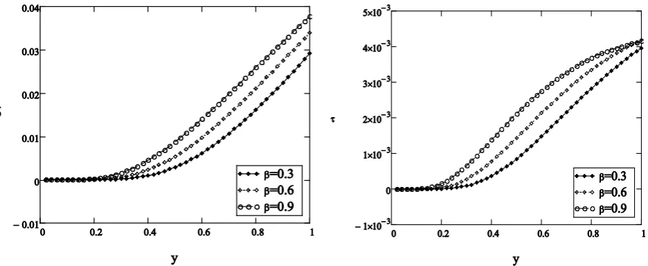
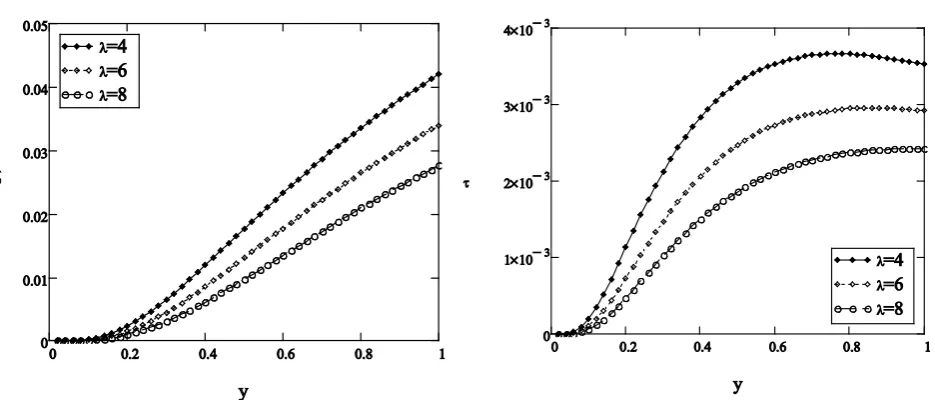
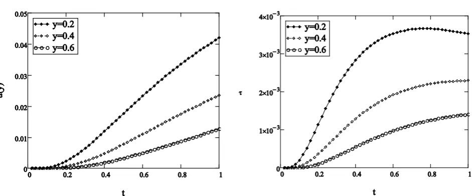
The effects of fractional parameters β of the model are important for us to be discussed. In Figure 1 we depict the profiles of velocity and shear stress for three different values of β. It is observed from these figures that the flow velocity as well as the shear stress increases with increasing β, which corresponds to the shear thinning phenomenon. Figure 2 are sketched to show the velocity and the shear stress profiles at different values of λ. It is noticeable that velocity as well as the shear stress decreases by increasing λ. In order to study the effects of materi-al parameter θ, we have plotted Figure 3, where it appears that the velocity is al-so a strong function of the material parameter θ of Jeffrey fluid. It can be ob-served that the increase of material parameter θ acts as an increase of the mag-nitude of velocity components near the plate, and this again corresponds to the shear-thinning behavior of the examined non-Newtonian fluid. Figure 4
[image:8.595.67.535.498.690.2]presents, the velocity field and the shear stress profiles at different values of y. It
DOI: 10.4236/ajcm.2017.74029 410 American Journal of Computational Mathematics
Figure 2. Velocity u(y,z,t) and shear stress τ1(y,z,t) profiles given by Equations (16) and (23), K = 2, t = 4, h = 2, M = 0.3, θ = 3, ξ = 1.2, β = 0.6 and different values of λ.
Figure 3. Velocity u(y,z,t) and shear stress τ1(y,z,t) profiles given by Equations (16) and (23), K = 2, t = 4, h = 2, M = 0.3, β = 0.6, ξ = 1.2, λ = 6 and different values of θ.
is noticeable that velocity and shear stress decreases by increasing y. Also, by in-creasing y the velocity becomes steady, which shows that the boundary condi-tion (9) is satisfied.
10. Conclusion
[image:9.595.63.527.312.498.2]DOI: 10.4236/ajcm.2017.74029 411 American Journal of Computational Mathematics
Figure 4. Velocity u(y,z,t) and shear stress τ1(y,z,t) profiles given by Equations (16) and (23), K = 2, t = 4, h = 2, M = 0.3, θ = 3, ξ = 1.2, λ = 6, β= 0.6 and different values of y.
conditions have been obtained. The similar solutions for ordinary Jeffrey fluid, performing the same motion, appear as limiting case of the solutions are ob-tained here. Also, the obob-tained results are analyzed graphically through various pertinent parameters. Furthermore, the obtained solutions satisfy the governing equations and all imposed initial and boundary conditions.
References
[1] Rajagopal, K.R. and Srinivasa, A. (1995) Exact Solutions for Some Simple Flows of an Oldroyd-B Fluid. Acta Mechanica, 113, 233-239.
https://doi.org/10.1007/BF01212645
[2] Tan, W.C. and Masuoka, T. (2005) Stoke’s First Problem for Second Grade Fluid in a Porous Half Space. International Journal of Non-Linear Mechanics, 40, 515-522. https://doi.org/10.1016/j.ijnonlinmec.2004.07.016
[3] Tan, W.C. and Masuoka, T. (2005) Stoke’s First Problem for an Oldroyd-B Fluid in a Porous Half Space. Physics of Fluid, 17, 23-101. https://doi.org/10.1063/1.1850409 [4] Fetecau, C. and Fetecau, C. (2005) Starting Solutions for Unsteady Unidirectional
Flows of a Second Grade Fluid. International Journal Engineering Sciences, 43, 781-789. https://doi.org/10.1016/j.ijengsci.2004.12.009
[5] Fetecau, C, and Fetecau, C. (2005) Decay of Potential Vortex in an Oldroyd-B Fluid. International Journal of Non-Linear Mechanics, 43, 340-351.
https://doi.org/10.1016/j.ijengsci.2004.08.013
[6] Khadrawi, A.F., Al-Nimr, M.A. and Othman, A. (2005) Basic Viscoelastic Fluid Problems using the Jeffreys Model. Chemical Engineering Science, 60, 7131-7136. [7] Chen, C.I., Chen, C.K. and Yang, Y.T. (2004) Unsteady Uni-Directional Flow of an
Oldroyd-B Fluid in a Circular Duct with Different Given Volume Flow Rate. Inter-national Journal of Heat and Mass Transfer, 40, 203-209.
https://doi.org/10.1007/s00231-002-0350-7
[8] Podlubny, I. (1999) Fractional Differential Equations. Academic Press, San Diego. [9] Hilfer, R. (2002) Applications of Fractional Calculus in Physics. World Scientific
DOI: 10.4236/ajcm.2017.74029 412 American Journal of Computational Mathematics [10] Bagley, R.L. and Torvik, P.J. (1986) On the Fractional Calculus Model of
Viscoelas-tic Behavior. Journal of Rheology, 30, 133-155.https://doi.org/10.1122/1.549887 [11] Friederich, C. (1991) Relaxation and Retardation Functions of the Maxwell Model
with Fractional Derivatives. Rheologica Acta, 30, 151-158.
https://doi.org/10.1007/BF01134604
[12] Li, J. and Jiang, T.Q. (1993) The Research on Viscoelastic Constitutive Relationship Model with Fractional Derivative Operator. South China Technology University Press. [13] Tong, D., Wang, R. and Yang, H. (2005) Exact Solutions for the Flow of
Non-Newtonian Fluid with Fractional Derivative in an Annular Pipe. Science China Physics, Mechanics & Astronomy, 43, 485-495.https://doi.org/10.1360/04yw0105 [14] Qi, H. and Xu, M. (2007) Stokes’ First Problem for a Viscoelastic Fluid with the
Generalized Jeffrey Model. Acta Mechanica Sinica, 23, 463-469.
https://doi.org/10.1007/s10409-007-0093-2
[15] Khan, A. and Zaman, G. (2016) The Oscillating Motion of a Generalized Oldroyd-B Fluid in Magnetic Field with Constant Pressure Gradient. Special Topics & Reviews in Porous Media, 6, 251-260.
https://doi.org/10.1615/SpecialTopicsRevPorousMedia.v6.i3.30
[16] Fetecau, C., Fetecau, C., Khan, M. and Vieru, D. (2008) Decay of a Potential Vortex in a Generalized Oldroyd-B Fluid. Applied Mathematics and Computing, 205, 497-506.
[17] Khan, A. and Zaman, G. (2017) Hydromagnetic Flow Near an Accelerating Plate in the Presence of Magnetic Field through Porous Medium. Georgian Mathematical Journal.https://doi.org/10.1515/gmj-2017-0017
[18] Khan, A. and Zaman, G. (2015) The Motion of a Generalized Oldroyd-B Fluid be-tween Two Side Walls of a Plate. South Asian Journal of Mathematics, 5, 42-52. [19] Khan, A., Zaman, G. and Rahman, G. (2015) Hydromagnetic Flow near a
Non-Uniform Accelerating Plate in the Presence of Magnetic Field through Porous Medium. Journal of Porous Media, 18, 801-809.
https://doi.org/10.1615/JPorMedia.v18.i8.50
[20] Khan, A. and Zaman, G. (2016) Unsteady Magneto-Hydrodynamic Flow of Second Grade Fluid Due to Uniform Accelerating Plate. Journal of Applied Fluid Mechan-ics, 9, 3127-3133.
[21] Khan, Z.H. and Khan, W.A. (2008) N-Transform-Properties and Applications. NUST Journal of Engineering Sciences, 1, 127-133.
[22] Belgacem, F.B.M. and Silambarasan, R. (2012) Theory of the Natural Transform. Mathematics in Engineering Science and Aerospace, 3, 99-124.
[23] Maitama, S. (2016) A Hybrid Natural Transform Homotopy Perturbation Method for Solving Fractional Partial Differential Equations. International Journal of Diffe-rential Equations, 2016, 8-15.https://doi.org/10.1155/2016/9207869
[24] Loonker, D. and Banerji, P.K. (2013) Solution of Fractional Ordinary Differential Equations by Natural Transform. International Journal of Mathematics and Engi-neering Science, 12, 1-7.
[25] Rawashdeh, M.S. and Maitama, S. (2015) Solving Nonlinear Ordinary Differential Equations using the NDM. Journal of Applied and Analytic Computations, 5, 77-88. [26] Mathai, A.M., Saxena, R.K. and Haubold, H.J. (2010) The H-Functions: Theory and
Applications. Springer, New York.https://doi.org/10.1007/978-1-4419-0916-9 [27] Hayat, T., Khan, M., Fakhar, K. and Amin, N. (2010) Oscillatory Rotating Flows of a
Fractional Jeffrey Fluid Filling a Porous Space. Journal of Porous Media, 13, 29-38.