Munich Personal RePEc Archive
Effects of foreign aid on the recipient
country’s economic growth
Pham, Ngoc-Sang and Pham, Thi Kim Cuong
Montpellier Business School, BETA, University of Strasbourg
18 April 2019
Online at
https://mpra.ub.uni-muenchen.de/93379/
Effects of foreign aid on the recipient country’s
economic growth
∗
Ngoc-Sang PHAM
a†and
Thi Kim Cuong PHAM
b‡a
Montpellier Business School, France
b
BETA, University of Strasbourg, France
April 18, 2019
Abstract
We introduce an infinite-horizon endogenous growth framework for studying the effects of foreign aid on the economic growth in a recipient country. Aid is used to partially finance the recipient’s public investment. We point out that the same rule of aid may have very different outcomes, depending on the recipient’s circumstances in terms of development level, domestic investment, efficiency in the use of aid and in public investment, etc. Foreign aid may promote growth in the recipient country, but the global dynamics of equilibrium are complex (because of the non-monotonicity and steady state multiplicity). The economy may converge to a steady state or grow without bounds. Moreover, there are rooms for the divergence and a two-period cycle. We characterize conditions under which each scenario takes place. Our analysis contributes to the debate on the nexus between aid and economic growth and in particular on the conditionality of aid effects.
Keywords: Aid effectiveness, economic growth, cycle, poverty trap, public invest-ment, threshold.
JEL Classification: H50, O19, O41
1
Introduction
Since the United Nations Summit in September 2000 at which the Millennium Develop-ment Goals (MDGs) were agreed, foreign aid, in particular, Official DevelopDevelop-ment Assis-tance (ODA) has been continually increasing. For example, in 2015, development aid provided by the donors in the OECD Development Assistance Committee (DAC) was 131.6 billion USD, increased by 6.9% in real terms from 2014, and by 83% from 2000.
∗The authors are very grateful to an Associate Editor and two anonymous referees for useful comments
and suggestions. They have helped us to substantially improve our previous version. We thank Laurent Wagner, Antoine Leblois and the participants at 18th Annual Meeting of the Association for Public Economic Theory, the 2016 Annual Conference of the Public Choice Society, the 65th Annual Meeting of the French Economic Association (AFSE), the 9th VEAM and the 2nd Workshop ”Sustainability”, the 17th Journ´es Louis-Andr´e G´erard-Varet and the Journ´ee du BETA for comments and suggestions.
At the same time, bilateral aid, provided by one country to another, risen by 4% in real terms.1 Many issues are under debate regarding the effectiveness of aid in terms of
economic growth. Indeed, extensive empirical investigations using different data samples show conflicting results.
On the one hand, some studies show that aid may exert a positive and conditional effect on economic growth. In a seminal paper Burnside and Dollar(2000) use a database on foreign aid developed by the World Bank and find that foreign aid has a positive effect on growth only in recipient countries which have good fiscal, monetary and trade policies.
Collier and Dollar (2001, 2002) use the World Bank’s Country Policy and Institutional Assessment (CPIA) as a measure of policy quality and show that aid may promote eco-nomic growth and reduce the poverty in recipient countries if the quality of their policies is sufficiently high. The findings in Guillaumont and Chauvet (2001),Chauvet and Guil-laumont (2003, 2009) indicate that the marginal effect of aid on growth is contingent on the recipient countries’ economic vulnerability. While economic vulnerability is negatively associated with growth, the marginal effect of aid on growth is an increasing function of vulnerability.
On the other hand, other empirical studies, not rejecting the conditionality of aid effects, show a certain fragility of results and suggest a non-linear effect of aid on growth (Hansen and Tarp, 2001; Easterly et al., 2004; Islam, 2005; Roodman, 2007; Clemens et al.,2012;Guillaumont and Wagner,2014). For example,Islam(2005) shows an aid Laffer curve in recipient countries with political stability. The effect of aid on growth may be negative at a high level of aid inflows. Hansen and Tarp(2001) find that the effectiveness of aid is conditional on investment and human capital in recipient countries and aid has no effect on growth when controlling for these variables. Their findings shed light on the link between aid, investment, and human capital and show that aid increases economic growth through its impact on capital accumulation. Using the same empirical specification like that in Burnside and Dollar (2000), but expanding the data set sample, Easterly et al.
(2004) nuance the claim from that of these authors. The results on aid effectiveness seem to be fragile when varying the sample and the definition of different variables such as aid, growth and good policy (Easterly, 2003).
The aforementioned conflicting results in the literature raise a concern about the effec-tiveness of foreign aid. Our paper deals with this concern by investigating the following questions: (1) How the recipient country use foreign aid to enhance economic growth? (2) What are the determinants of the effectiveness of foreign aid? (3) Why are the effects of foreign aid significant for some countries but not for others?
To address these questions, we consider a tractable discrete-time infinite-horizon growth model where public investment, which is financed by foreign aid and capital tax, may im-prove the total factor productivity (TFP) if it is large enough. Inspired by the empirical literature, we formulate aid flows taking into account the donor’s rules and the recipient’s need represented by its initial capital stock. In the case of a poor country, we also con-sider the efficiency in the use of aid and in public investment, then examine their impacts on the aid effectiveness. Our model allows us to find explicitly the dynamics of capital stocks, and provide a full analysis of equilibrium transitional dynamics. We show that if the initial circumstances of the recipient are good enough (high productivity and initial capital), the country does not need foreign aid to achieve its development goals. This
1For more information, see
result is in line with the findings in growth models with increasing return to scale. Con-sequently, our analysis focuses on the case in which the recipient country’s initial capital and productivity are not high. The main results can be described as follows:
First, when the foreign aid is very generous and/or the use of aid is efficient, and the recipient country has a high quality of circumstances (high and efficient public investment and/or low fixed cost in public investment), then the economy will grow without bounds for any level of initial capital stock. Consequently, the country will no longer receive aid from some date on.
The second case, corresponding to the richest dynamics of equilibrium, is found when foreign aid is not very generous and the recipient has an intermediate quality of circum-stances. In this case, we distinguish 2 regimes: (R1) the recipient country focuses on its domestic investment, characterized by a remarkable level of capital tax financing public investment, and (R2) it focuses on foreign aid, characterized by the fact that the use of foreign aid is sufficiently efficient. In the first regime (domestic investment focus), if the country has sufficient initial capital or/and the foreign aid is quite high, the economy can grow. Otherwise, it would collapse (i.e., the capital level tends to zero) or stay at the unique steady state. In the second regime, the transitional dynamics are complex because of the non-monotonicity of capital dynamics. The non-monotonicity is due to the fact that the country focuses on foreign aid which decreases when the economy gets better. In this regime, there are two steady states: the lower one is interpreted as a middle-income trap while the second one as a poverty trap. Let us present our findings under this regime R2.
R2.1. We prove that any poor country, receiving a middle-level aid flow and using it efficiently, always grows at the first stage of its development process and hence will never collapse. This is intuitive because if the capital stock is very low, the country receives a significant aid flow which improves its investment. Under mild conditions, we show that the economy can increasingly converge to the low steady state.
R2.2. However, the convergence may fail in some cases and there may exist a two-period cycle capital path. The intuition is the following: When a poor country receives aid at an initial date (date 0), its economy may grow at date 1. By the rule of aid, the aid flow for date 1 may decrease, leading to a decrease of total public investment at date 1. Hence, the capital at date 2 may decrease, and so on. Thus, a two-period cycle may arise.
R2.3. Last, we point out that a poor country, having strong dynamics of capital, can take advantage of foreign aid to finance its public investment. This may lead it to overcome the middle-income trap in a finite number of periods and to obtain growth in the long run. In this case, the recipient will no longer receive aid from some date on.2
Several empirical studies on the effects of aid and conditionality of aid effectiveness in different recipient countries may illustrate our theoretical analyses. First, South Korea offers an illustration for our results in regime R1 and regime R2.3. Indeed, this country was a recipient country during the period of 1960-1990 (after the Korean War 1950-1953) and experienced a high domestic investment during this period. South Korea is now
2Strong dynamics of capital are defined in our paper in the sense that there is some value of capital
a developed country and has become a member of the OECD-DAC (since 2010). The average aid flows have decreased during the period of 1960-1980, from 6.3% to 0.1% of GDP. It became negative at the beginning of the 1990s.3 Second, our analysis in the
regime R2.1 may be illustrated by the Tunisia case where aid flows have also decreased during 1960-2003, from 8.1% of GDP in the 1960s to 1.5% during 1990-2003.4
From a theoretical point of view, our paper is closely related to Dalgaard (2008) who considers that aid flows depend on the recipient’s income per capita and on the donor’s exogenous degree of inequality aversion. However, there are some differences. First,
Dalgaard (2008) considers an OLG growth model while we use an infinite-horizon model `a la Ramsey. Second, in Dalgaard(2008), public investments are fully financed by foreign aid while in our paper public investments are financed, not only by foreign aid but also by capital tax. In Dalgaard(2008), the transitional dynamics of capital stock are totally determined by the degree of inequality aversion on the part of the donor. Our contribution is to show that the transitional dynamics depend not only on the aid rule but also on the country’s characteristics. In particular, our framework allows us to study whether a poor country can surpass, not only the low steady state but also the high one and then achieve growth in the long run.
Our theoretical results complemented by a number of numerical simulations, indicate that the effects of aid (in the short run and in the long run) are complex, non-linear and conditional on recipient countries’ characteristics. By the way, our paper is related to and complements the points in Charterjee et al. (2003), Charteerjee and Tursnovky (2007). Indeed, Charterjee et al. (2003) examine the effects of foreign transfers on the economic growth of the recipient country given that foreign transfers are positively proportional to the recipient’s GDP but are not subject to conditions. They show that their effects on growth and welfare are different according to the type of transfers, untied or tied to investment in public infrastructures. Charteerjee and Tursnovky (2007) underly the role of endogeneity of labor supply as a crucial transmission mechanism for foreign aid.
Our paper is likewise related to the literature on optimal growth with increasing returns (Romer, 1986; Jones and Manuelli, 1990; Kamihigashi and Roy, 2007) and with the presence of threshold (Azariadis and Drazen, 1990; Bruno et al., 2009; Le Van et al., 2010, 2016). Different from numerous papers in this literature, we point out the role of aid which can provide investment for the least developed country, this helps the recipient country to evade poverty and potentially obtain positive growth in the long run. Moreover, policy function in our framework may not be monotonic.
The remainder of the paper is organized as follows. Section 2 characterizes the case of a small recipient country. Section 3presents the dynamics of capital, in particular, the poverty trap without international aid. In Section 4, we emphasize the role of foreign aid by analyzing the conditions for the effectiveness of aid. Section 5 studies effects of aid in a centralized economy. Section 6 concludes. Technical proofs are presented in Appendix
A.
2
A small economy with foreign aid
This section presents our framework. We consider an economy with infinitely-lived iden-tical consumers and a representative firm. The population size is constant over time and normalized to unity. Labor is exogenous and inelastic. The representative firm produces a single good, which can be used for either consumption or investment. The government uses capital tax and foreign aid to finance public investment (including R&D investment) which can improve the total factor productivity. The waste in aid spending is considered by the presence of unproductive aid. The latter has no direct effect on the household’s welfare, nor on the production process. The fraction of wasteful aid may reflect the degree of inefficiency (including corruption) in the use of aid.
2.1
Foreign aid and public investment
The literature on aid conditionalities has a large consensus on the recipient’s need as a significant criterion of aid allocation: countries with a high need should receive a high amount of aid. This criterion, among others, is used in several bilateral and multilateral aid policies. For instance, the World Bank’s International Development Association (IDA) uses a specific rule of aid allocation which gives priority to the poorest countries and also those with the ability to use aid effectively. Compared to the IDA, the Asian Development Bank formula assigns a higher weight to recipient countries’ poverty, but a lower weight to the recipient’s population size.5 In a study for the 2008 Development Cooperation
Forum at the UN Economic and Social Council, Andersson(2008) (Box 1 and Figure 7) evoked different factors, including initial income, influencing the form of aid allocation. Other studies (Carter, 2014; Guillaumont and Wagner, 2015; McGillivray and Pham,
2017) provided more details on these aid allocation rules and mentioned a formula of aid allocated to a recipient country as a function of its poverty.
In this sense, we can assume that aid per capitaat takes the following form:
at= (¯a−φkt)+ ≡max{¯a−φkt,0} (1)
where ¯a > 0, the maximal aid amount that the recipient country can receive, and φ, independent of the per capita capital, may be referred to all exogenous rules imposed by the donor.
Equation (1) means that the higher the per capita capital kt, the lower the country
ranks in its need, then the lower the aid received. A similar assumption may be found in
Carter (2014) andDalgaard (2008).6 The form of equation (1) implies that a decrease in
φ and/or an increase in ¯a lead(s) to a higher aid flow. Moreover, from a threshold (¯a/φ)
5Other international institutions such as the Asian Development Bank, the European Development
Fund, the UK’s Department for International Development, etc. use different variants of this rule.
6Carter (2014) (page 135) considers that aid flow received by country iis positively correlated with
country performance rating as underlined inCollier and Dollar(2001,2002) (with index Country Policy and Institutional Assessment) and is negatively associated with income per capita. Dalgaard (2008) assumes that per capita flow of aid at timetis also a reversed function of income of per capita at period (t−1), at = θytλ−1, where θ > 0 and λ < 0. In this aid function, λ reflects the degree of inequality
aversion of the donor. Parameterθrepresents exogenous determinants of aid. Although Appendix C.2 in
Dalgaard(2008) presents a generalized aid allocation rule, it seems that this rule does not cover the form of (1) because the function (¯a−φx)+is not differentiable. Our analyses of effects of threshold (¯a/φ) are
of capital, the recipient country no longer receives aid. In Section 4.5, we will work under a general form of aid.
The positive couple (¯a, φ) is interpreted as the aid rule imposed by the donor. It is taken as given by the recipient country and represents aid conditionalities. Allocation of aid may be conditional on the policy performance as underlined in Burnside and Dollar
(2000),Collier and Dollar(2001,2002). According to these authors, a country with a high policy quality is more able to use aid in an efficient way. Guillaumont and Chauvet(2001) focus on a fairness argument when they focus on the recipient’s economic vulnerability: more aid should be provided to countries with a high economic vulnerability since in these countries aid would be more efficient. This argument also fits in a philosophy of fairness which proposes that aid should compensate the recipient country for its vulnerable initial situation (in macroeconomic conditions or lack of human capital), so that all countries can begin at the same initial opportunities. McGillivray and Pham (2017), Guillaumont et al. (2017) consider the lack of human capital as a determinant criterion. Other analyses underline the link between aid and political variables (strategic allies, former colonial status, and the ability to use aid effectively), between aid and macroeconomic conditions (trade openness, commercial allies, etc.) (Alesina and Dollar, 2000; Berthelemy and Tichit,2004). All these factors are exogenous for the recipient country as they are chosen by donors and may be considered as different interpretations of the parameterφ. Equation (1) may reflect a trade-off between needs (low initial capital) and country-selectivity (high
φ) or a compatibility between needs (low initial capital) and country-selectivity (low φ) based on aid performance or other criteria.
The recipient country uses aid and tax on capital to finance public investment which improves private capital productivity. Since some spending of aid is wasted in most recipient countries, there is a significant part of the unproductive activity, noted as au
t.
This is potentially explained by corruption, administrative fees, etc. Then, the attribution of aid may be written as:
at=ait+a u
t (2)
where ai
t represents the part of aid which contributes to the public investment of the
recipient country. If we consider a fixed fraction of aid for each activity, we can rewrite equation (2) as follows:
at =αiat+αuat
with αu = 1−αi. Parameter αu ∈(0,1) reflects the degree of inefficiency (including the
corruption) in the use of aid while αi represents the efficiency in the use of aid.
Let us denoteBt the public investment financed by tax on capital and by aid,Btmay
be written as:
Bt=Tt−1+ait (3)
where Tt−1 is the tax at periodt−1. We assume that Tt−1 =τ Kt used to finance public
investment which will have its effect at datet. Since, all capital tax is used to fund public investment,τ may be interpreted as the government effort in financing public investment.7
7The amount T
t=τ Kt+1 in our model can be viewed as the total expenditure in R&D which may
The positive effect of foreign aid on public investment is an obvious finding in empirical studies (Khan and Hoshino, 1992; Franco-Rodrigez et al., 1998; Ouattara, 2006; Feeny and McGillivray, 2010).
2.2
Production with endogenous productivity
At each date, the representative firm maximizes its profit. The production function at date t is given by Ft(Kt) = AtKt where Kt represents the capital whileAt represents the
total factor productivity. In the spirit of Barro(1990), we assume that At is endogenous
and depends on public investment Bt as follows:
At≡A
1 + (σBt−b)+
. (4)
Parameter A ∈ (0,∞) is interpreted as autonomous productivity. Parameter σ ∈
(0,∞) measures the extent to which the public investment translates into technology and it reflects the efficiency of public investment. So, σBt can be viewed as a flow of
new technology/innovation generated by the investmentBt. Parameterb is the threshold
from which the flow of technology σBt has a strictly positive impact on the TFP. The
threshold b may be viewed as a fixed cost or setup cost (Azariadis and Drazen, 1990).8
When Bt ≤b/σ, we have (σBt−b)+= 0, and thenAt =A. This means that the positive
effect of public investment on total productivity is observed only from the level b/σ. In Section 4.5, we will work under a general form of TFP At.
According to (3) and (4), foreign aid has a significant effect on the capital productivity and production only if ai
t ≥ b/σ −τ Kt. As in Charterjee et al. (2003), Charteerjee
and Tursnovky (2007), Dalgaard (2008), we consider that aid is used to finance public expenditures. However, for countries with low capital (in the sense that στ Kt < b),
aid should be higher than a critical level to improve the technology which is necessary for positive growth in the long run.9 This assumption may be referred to the big push
concept of aid supported by Sachs(2005) and discussed inGuillaumont and Guillaumont Jeanneney (2010). Our setup is also supported by Wagner (2014) who uses a database including 89 recipient countries and identified the existence of a critical level above which aid is effective in terms of economic growth.
At each periodt, givenBt, rt, the representative firm maximizes its profit:
(Pf t) : πt≡max Kt≥0
Ft(Kt)−rtKt
It is straightforward to obtain rt and πt for a competitive economy:
rt =A
1 + σBt−b +
and πt= 0. (5)
Remark 1. We may introduce a more general setup
A′t≡A h
1 + σ(Bt−b1)+−b2
+i
. (6)
8Our setup (4) is related to that inBruno et al. (2009). The role ofb(resp.,σBt)in our framework is
similar to that of the parameterX (resp.,Ye,t) inBruno et al.(2009).
9Our setup is different from that inDalgaard(2008). Indeed,Dalgaard(2008) considers a production
function: yt=kαtg1− α
where ¯b1 represents the fixed cost due to, for example, bribery and b2 plays the role of
b in (4). Notice that A′ t = A
1 + σBt−b)+
where b ≡ σb1+b2. So, our main results
still hold under this general setup. However, there is a difference in terms of implications which will be discussed in Remark 3.
2.3
Household
Let us consider the representative consumer’s optimization problem. She maximizes her intertemporal utility by choosing consumption and capital sequences (ct, kt):
(Pc) : max
(ct,kt+1)+
∞
t=0 +∞ X
t=0
βtu(ct)
s.t: ct+kt+1+Tt ≤(1−δ)kt+rtkt+πt
where k0 >0 is given, β is the rate of time preference and u(·) is the consumer’s
instan-taneous utility function. Tt is the tax, rt is the capital return while πt is the firm’s profit
at date t.
For the sake of tractability, we assume that the consumer knows thatTt=τ kt+1 and
instantaneous utility function is logarithmic, u(ct) = ln(ct). According to Lemma 8 in
Appendix A.1, we establish the relationship betweenkt+1 and kt
kt+1 =β
1−δ+rt
1 +τ kt. (7)
Since the utility function is strictly concave, the solution is unique.
2.4
Intertemporal equilibrium
Definition 1 (intertemporal equilibrium). Given tax rate τ, a list (rt, ct, kt, Kt, at) is an
intertemporal equilibrium if:
1. (ct, kt) is a solution of the problem Pc, given ait, rt, πt.
2. (Kt) is a solution of the problemPf t, given Bt and rt.
3. (Market clearing conditions) Kt =kt and ct+kt+1+Tt = (1−δ)kt+Yt.
4. The government budget is balanced: Tt=τ kt+1.
5. (Rule of Aid) at = max{¯a−φkt,0} and ait=αiat.
Combined with (5), the dynamics of capital stock may be rewritten as follows:10
kt+1 =G(kt)≡f(kt)kt (8a)
where f(kt)≡β
1−δ+Ah1 + σ(τ kt+αi(¯a−φkt)+)−b +i
1 +τ . (8b)
This dynamic system is non-linear and non-monotonic. The next sections analyze the global dynamics of capital stocks (kt) and the effects of international aid on the recipient’s
economic growth. Before doing this, it is useful to introduce some notions of growth and collapse.
10We implicitly assume that P
tβ
tu(Gt(k
0)) < ∞ where G0(k0) ≡ k0 and Gt+1(k0) = G(Gt(k0))
Definition 2 (growth, collapse, and poverty trap).
1. The economy collapses if limt→∞kt= 0. It grows without bounds if limt→∞kt=∞.
2. A value ¯k is called a trap if, for any initial capital stockk0 <k¯, we have kt<¯k for
any t high enough.
Our formal definition of trap means that a poor country (k0 ≤ k¯) continues to be
poor. It is in line with the notion of poverty trap in Azariadis and Stachurski(2005): A poverty trap is a self-reinforcing mechanism which causes poverty to persist.
3
Equilibrium dynamics without foreign aid
This section considers an economy which does not receive foreign aid. Its public invest-mentBtis entirely financed by tax revenue. We will analyze the transitional dynamics of
capital. From equation (8a), we have:
kt+1=fb(kt)kt, wherefb(kt)≡β
1−δ+Ah1 + στ kt−b +i
1 +τ (9)
Let us denote:
ra≡β
1−δ+A
1 +τ . (10)
We observe fb(kt)≥ra for any t. Therefore, we have:
Remark 2(role of autonomous technology). Consider an economy without aid. Ifra>1,
the economy will grow without bounds.11
Conditionra >1 is equivalent to A > 1+βτ +δ−1. If we define the subjective interest
rate ρ by (1 +ρ)β = 1, then 1+τ
β +δ−1 = (1 +τ)(1 +ρ) +δ−1≈τ +ρ+δ which can
be interpreted as the investment cost. By consequence, condition ra >1 means that the
autonomous productivity is higher than the investment cost. Under this condition the economy will have growth whatever the levels of other factors such as: initial capital or efficiency of public investment. In this case, the country does not need foreign aid to get economic growth. Since our purpose is to look at the impacts of public investment and foreign aid, from now on, we will work under the following assumption.
Assumption 1 (for the rest of the paper). ra≤1 or equivalently,
A ≤ 1+τ
β +δ−1.
Under this assumption, the economy would never reach economic growth in the long run without public investment Bt (in infrastructure, in R&D program, etc.). Public
investment Bt is then required to improve technology, and this is necessary for a positive
economic growth in the long run.
According to equation (9) and the fact that fb(kt) is an increasing function, we get
the following properties concerning the dynamics of capital stock:
11In this case,fb(kt)≥r
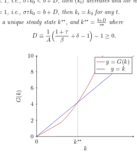
Proposition 1 (poverty trap and growth: role of public investment). Consider an econ-omy with a low level of autonomous technology (Assumption 1 holds), and without foreign aid. The public investment in technology is entirely financed by tax revenue. The dynamics of capital, characterized by equation (9), are as follows:
1. If fb(k0)>1, i.e., στ k0 > b+D, then(kt)increases and the economy grows without
bounds.
2. If fb(k0)<1, i.e., στ k0 < b+D, then (kt) decreases and the economy collapses.
3. If fb(k0) = 1, i.e., στ k0 =b+D, then kt =k0 for any t.
There exists a unique steady state k∗∗, and k∗∗= b+D
τ σ where
D ≡ 1
A
1 +τ
β +δ−1
−1≥0. (11)
0 0 2 4 6 8 10
k∗∗
k
G
(
k
)
y=G(k)
[image:11.628.168.441.196.499.2]y=k
Figure 1: Transitional dynamics of capital without foreign aid and ra <1.
We may interpret b as a fixed cost of public investment. If the return of public investment (σBt ≡ στ k0), also interpreted as the flow of new technology, is less than
b+D, public investmentτ k0 does not make any change to the total factor productivity.
Following this interpretation, b+D can be viewed as the threshold so that if the return of public investment in R&D (σBt) is less than this level, there is no growth of capital
stock, i.e. kt+1 < kt for all t.
Figure1illustrates Proposition1.12 The point of interaction between the convex curve
and the first bisector corresponds to the unstable steady state k∗∗ which is considered as
a poverty trap for this economy (see Definition 2). For all initial capital k0 higher than
k∗∗ (corresponding toστ k
0 > b+D), the economy will grow without bounds while it will
collapse if the initial capital is lower than k∗∗. It should be noticed thatk∗∗ is decreasing
in A, σ but increasing in b. This means that an economy having a high autonomous technology A, high efficiency σand low fixed cost bin public investment, obtains a higher probability to surpass its poverty trap as the condition στ k0 > b+Dis more likely to be
satisfied.
4
Equilibrium dynamics with foreign aid
Point 2 of Proposition 1 shows that the economy collapses without international aid if
στ k0 < b+D. Since we want to investigate the effectiveness of aid, we will work under
the following assumption in Section 4:
Assumption 2 (for the whole Section 4).
στ k0 < D+b (12)
where D is defined by (11)
Given this pessimistic initial situation of the recipient country, we examine how in-ternational aid could generate positive perspectives in the short run as well as in the long run. Recall that kt+1 = G(kt). Before exploring the dynamics of capital stock, it is
essential to underline properties of function f(k) and G(k). To do so, we introduce some notations
x1 ≡¯a/φ, x2 ≡
σαi¯a−b
σ(αiφ−τ)
, x3 ≡
1−δ+A(1 +σαia¯−b)
2Aσ(αiφ−τ)
. (13)
Let us explain the meaning of x1, x2, x3. First, x1 is the maximum level of capital
stock so that the recipient country does not receive international aid. Second, when the country receives aid, x2 is the critical threshold from which public investment Bt
(financed by aid and tax revenue) has a positive impact on productivity (x2 is a solution
toσ τ k+αi(¯a−φk)
−b) = 0. Last, when the country receives aid (i.e., ¯a−φk >0) and public investment has positive impact on productivity (i.e., σ τ k+αi(¯a−φk)
−b >0),
x3 is a local-maximum point of function G (because f3′(x3) = 0) where
f3(x)≡β
1−δ+Ah1 + σ(τ x+αi(¯a−φx))−b i
1 +τ x. (14)
Lemma 1 (increasingness of G). The function G is increasing on [0,∞) if one of the following conditions is satisfied.
1. τ ≥αiφ.
2. τ < αiφ and σαia < b¯ (which imply that x2 <0).
3. τ < αiφ, σαi¯a > b and x3 >min(x1, x2).
Condition τ ≥ αiφ means that the government effort is high (τ is high or/and αi is
low). In this case, the policy function is increasing. In point 2, the policy function G
is also increasing because the flow of aid αi(¯a−φx)+ plays no role on the endogenous
productivity. Conditions in point 3 mean that the government effort is low, the maximum level of aid ¯aand/or the efficiency of public investmentσis high with respect to the fixed cost b, and the local-maximum point of output is high enough.
When the local-maximum point is not high enough, the policy functionGmay not be increasing.
Lemma 2(non-monotonicity ofG). Assume thatτ < αiφ,σαi¯a > b, andx3 <min(x1, x2).
Proofs of Lemmas1, and 2 are presented in AppendixA.2.
We can find non-trivial fixed points (capital steady states) by computing strictly pos-itive solutions of the equation G(k) = k, or equivalentlyf2(k)≡τ k+αi(¯a−φk)+= Dσ+b.
Lemma 3 (steady states).
1. If σa¯min(αi, τ /φ)> D+b, then there is no fixed point.
2. Consider the case where σ¯amin(αi, τ /φ)≤D+b.
(a) If τ > αiφ, which implies σ¯aαi ≤D+b, then the unique fixed point is
(
k∗ ≡
D+b σ −¯aαi
τ−αiφ ∈(0,¯a/φ) if σ¯aτ /φ > D+b
k∗∗ ≡ D+b
τ σ ∈(¯a/φ,∞) if σ¯aτ /φ < D+b.
(15)
(b) If τ < αiφ, which implies σ¯aτ /φ≤D+b, then
i. If σ¯aαi < D+b, then the unique fixed point is k∗∗≡ Dτ σ+b ∈(¯a/φ,∞).
ii. If σaα¯ i > D+b, then there are two fixed points k∗ ≡
¯
aαi− D+b
σ
αiφ−τ ∈ (0,¯a/φ)
and k∗∗≡ D+b
τ σ ∈(¯a/φ,∞).
13
Proof. See Appendix A.2.14
4.1
Growth under high-quality circumstances
This section investigates effects of aid on the recipient prospects when the recipient coun-try has high-quality circumstances in terms of efficiency in the use of aid, fixed cost and efficiency in public investment, autonomous technology, etc.
Proposition 2 (growth without bounds thanks to foreign aid). Considering an aid re-cipient under a poverty trap without aid, characterized by condition (12). The dynamics of capital with foreign aid are characterized by (8a).
If
rd≡
β
1 +τ
h
1−δ+A1 + σ¯amin(αi, τ /φ)−b +i
>1
or equivalently, σ¯amin(αi, τ /φ)> D+b, (16)
then we have that,
1. the economy will grow without bounds for any level of initial capital k0,
2. international aid at = (¯a−φkt)+ decreases in t. Consequently, there exists a time
T such that aid flows at = 0 for any t≥T.
13Conditionσ¯aα
i> D+bensures thatk∗>0.
14In AppendixA.2, we also study the case whereτ=α
Proposition 2 can be proved by using point 4 of Lemma 1 and point 1 of Lemma 3. Notice that in this case, G is increasing and a steady state does not exist.
Condition (16) in Proposition 2may be written as follows
σ¯aτ
φ > D+b and σαia > D¯ +b, (17)
where D is given by equation (11). Two conditions in (17) mean that the foreign aid is generous (high ¯a and lowφ) and/or the recipient country has high-quality circumstances (that is, a high efficiency σ and low fixed cost b in public investment, and/or a high level of autonomous technology A). In particular, the first condition in (17) may be associated with a high government effort (high τ) in financing public investment while the second condition may be associated with a high efficiency in the use of aid (high αi). In other
words, given aid flows and the donor’s rules characterized by the couple (¯a, φ), condition (17) is more likely to be satisfied if the recipient country has high-quality circumstances, decisive for the effectiveness of aid.
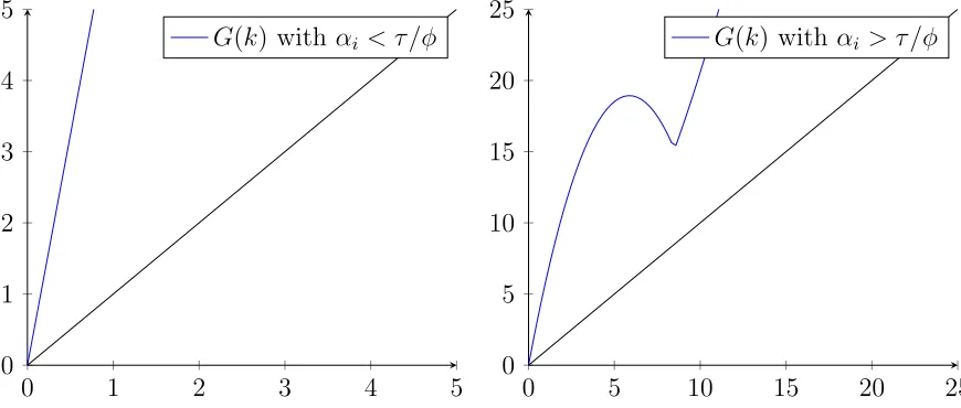
Proposition 2 presents the best and ideal scenario since whatever the initial capital, generous aid combined with high-quality circumstances could help the recipient country to grow without bounds in the long run. Figure2illustrates this proposition under condition (16).15 The graph on the left corresponds to the case α
i < τ /φ and that on the right
corresponds to the case αi > τ /φ. We observe that, without foreign aid (corresponding
to ¯a = 0), the dynamics of capital are similar to that in Figure1and there is one poverty trap. Thanks to development aid, the dynamics of capital change and they are represented by the curve above the first bisector.
0 1 2 3 4 5
0 1 2 3 4 5
G(k) with αi < τ /φ
0 5 10 15 20 25
0 5 10 15 20 25
[image:14.628.93.528.438.623.2]G(k) with αi > τ /φ
Figure 2: Growth without bounds. Conditions ra <1 and (16) holds
Remark 3. Assume that the TFP is A′
t := A[1 +σ(Bt−b1)+] instead of (4). Assume
also that αi¯a < b1, αiφ > τ and β1−δ1++τA <1. If x∈[0,¯a/φ], then we have
f(x) = β
1−δ+Ah1 +σαia¯−(αiφ−τ)x−b1
+i
1 +τ =β
1−δ+A
1 +τ <1.
15 Parameters in Figure 2 areβ = 0.8;τ = 0.4;δ= 0.2;A = 0.4;σ= 2;α
By consequence, we have limt→∞kt= 0 for anyk0 ≤a/φ¯ , whatever the level of efficiency
σ. This is different from Proposition 2 where limt→∞kt = 0 if σ is high enough. This is
due to the presence of threshold b1 which implies that A′t=A for any Bt ≤b1, whatever
the level of σ. We refer to Le Van et al. (2016) for endogenous threshold in an optimal growth model.
4.2
Growth or collapse? The role of aid
We are now interested in the case where condition (16) is not satisfied: recipient coun-tries do not have high-quality circumstances and/or aid flows, subject to conditions, are bounded, due to the budget constraint from the donors. In the next sections, we will work under the following condition:
Assumption 3 (for the rest of the paper).
σa¯min(αi, τ /φ)< D+b. (18)
From (18), we can identify three cases:
Low circumstances: στ
φ < D+b
¯
a and σαi < D+b
¯
a (19a)
Intermediate circumstances 1 (domestic investment focus): σαi <
D+b
¯
a < στ
φ (19b)
Intermediate circumstances 2 (aid focus): στ
φ < D+b
¯
a < σαi (19c)
In both (19b) and (19c), we have σa¯min(αi, τ /φ)< D+b < σ¯amax(αi, τ /φ). However,
we distinguish two intermediate circumstances: one with domestic investment focus when
αiφ < τ, that is the government investment (measured by τ) is quite high with respect to
the efficiency degree in the use of aid (measured by αi); and another with aid focus when
αi > τ /φ, that is the use of aid is quite efficient.
We firstly consider the cases of low circumstances and the domestic investment focus. According to Lemma 1, we have the following result.
Proposition 3 (growth or collapse? The role of aid). Consider an aid recipient under poverty trap without aid, characterized by condition (12): στ k0 < D+b. Assume that one
of three conditions in Lemma 1 holds. Then (kt) is monotonic in t and the transitional
dynamics of (kt) are characterized as follows.
1. If f(k0) > 1, i.e., σ(τ k0 +αi(¯a−φk0)+)−b
+
> D, then (kt) increases and the
economy grows without bounds. Consequently, there exists a time T such that aid flows at= 0 for any t≥T.
2. If f(k0) < 1, i.e., σ(τ k0+αi(¯a−φk0)+)−b
+
< D, then (kt) decreases and the
economy collapses. Consequently, there exists a time T1 such that aid flows at > 0
for any t≥T1.
Moreover, following Lemma 3, we have:
The unique steady state = (
k∗∗= D+b
τ σ ∈(¯a/φ,∞) if (19a) holds (low circumstances)
k∗ = ¯aαi− D+b
σ
αiφ−τ (0,¯a/φ) if (19b) holds (intermediate circumstances 1).
We are considering a country with a low initial capital stock in the sense thatστ k0 <
b+D(Assumption 2). According to Proposition3, we observe that: given such an initial capital stock k0, if the aid rule is generous (in the sense that ¯a is high and/or φ is low)
and the use of aid is efficient (αi is high) so that σ(τ k0+αi(¯a−φk0)+)−b
+
> D, then the economy will grow without bounds. Otherwise, the economy will collapse or stay at the steady state. In other words, the development aid might help the recipient to surpass its poverty trap while this is impossible without foreign assistance. Our result indicates that low-income and vulnerable countries need not only a large scaling-up of aid but also the efficiency in the use of aid (parameter αi) to help them to get out of the poverty trap.
Our finding may be considered as a theoretical illustration for the argument evoked in
Kraay and Raddatz (2007) using a Solow model.16
We observe that the poverty trap in the intermediate circumstances 1 (with domestic investment focus) is k∗, which is lower that k∗∗, i.e. the poverty trap in the low
circum-stances. This means that the intermediate circumstances give a better outcome than the low circumstances as the recipient’s possibility of escaping its poverty trap is higher in the intermediate circumstances.
4.3
Stability, fluctuations or take-off ? The complexity of aid’s
effects
We have so far analyzed three circumstances (high, low and intermediate circumstances 1 with domestic investment focus) in which the capital path (kt) is monotonic. In these
cases, the recipient country may or may not fully exploit the same flow of aid following its initial situation. This section focuses on the remaining cases characterized by the following assumption:
Assumption 4 (for the whole Section 4.3).
1. στ /φ < D+b
¯
a < σαi (condition (19c) - intermediate circumstances 2 with aid focus)
2. 0< x3 <min(x1, x2) where x1, x2, x3 are given by (13).
Assumption4means that: (1) the government investment is low (i.e. τ is low) but the use of aid is quite efficient (i.e. αi is quite hight); (2) the maximum level of aid ¯a and/or
the efficiency of public investment σ are quite high with respect to the fixed cost b, but the local-maximum point x3 of function G is not high enough (i.e. dynamics of capital
are not very strong) to surpass thresholds x1, x2. Notice that if Assumption4is violated,
we recover analyses in the previous sections.
16In a Solow model with two exogenous saving rates, there are two steady states which are locally
Under Assumption 4, G is not monotonic. It is increasing on [0, x3], decreasing on
[x3,min(x1, x2)], and increasing on [min(x1, x2),∞). By combining Assumption4, Lemma
2 and point (2.b.i) of Lemma 3, there exist two steady states :
low steady state k∗ = ¯aαi−
D+b σ
αiφ−τ
∈(0,¯a/φ), and high steady statek∗∗= D+b
τ σ ∈(¯a/φ,∞).
It is easy to see that the high steady state k∗∗ is unstable. The main question in this
section is whether the recipient country can encompass the high steady state and attain an economic take-off. It is also about to investigate whether the capital stock converges to the low steady state or fluctuates around it.
Let us start by considering a poor country (i.e., k0 is low).
Proposition 4. Assume that σαi¯a > D+b. When the initial capital stock k0 is low
enough, the capital stock at the next period will be higher than k0: k1 > k0.
Proof. Condition σαia > D¯ +bensures that f(0)>1. Since the functionf is continuous,
f(k0)>1 for any k0 low enough. By consequence, k1 =G(k0) =f(k0)k0 > k0.
Proposition4 leads to an important implication: any poor country (characterized by Assumption 4) receiving foreign aid and using it efficiently always grows at the first stage of its development process (see Figure 3 for an illustration, with k0 sufficiently far from
the low steady state). In this case, aid may not promote growth but the economy never collapses: this is an important difference between the case of intermediate circumstances with aid focus and the cases of low circumstances or intermediate circumstances with domestic investment focus (which may rise a collapse). It follows that we should provide development aid for such poor countries.
However, our result does not mean that we should provide more development aid for any country at any stage of its development. A natural question arises: What happens to poor or developing countries (having a low or middle value of k0)? We will address this
question in next subsections.
4.3.1 Stability and fluctuations
We start this section by considering the stability of capital path.
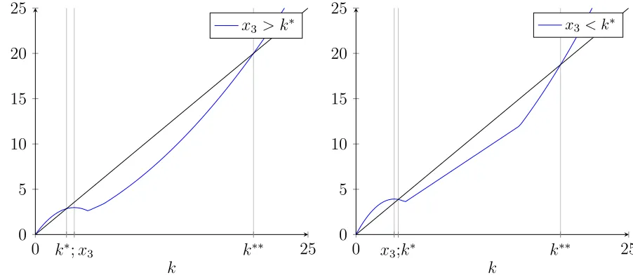
Proposition 5 (stability of low steady state). Let Assumption 4 be satisfied.
1. Considering the case where σaα¯ i < D+b+A1
1+τ β
, or equivalently x3 > k∗. We
have that: if k0 ∈(0, k∗), then kt∈(0, k∗) for any t and limt→∞kt=k∗.
2. Considering the case where σ¯aαi > D+b+A1
1+τ β
, or equivalently x3 < k∗. The
steady state k∗ is locally stable17 if and only if
σaα¯ i < D+b+
2
A
1 +τ
β
(20)
Proof. See Appendix A.3.
17It means that there existsǫ >0 such that limt
Recall that we are considering στ k0 < D+b, i.e., k0 < k∗∗ the country is in a situation
sufficiently vulnerable to have a possibility of collapse if there is no aid (according to point 1 of Proposition 1). Point 1 of Proposition 5 shows the role of aid: a country receiving development aid may converge to some point. This may happen under Assumption 4
and x3 > k∗, that is the low steady state is lower than the local-maximum point (x3)
of output. This finding complements Proposition 2 and Proposition 3: foreign aid may promote growth in the recipient country. It should be noticed that Propositions 2, 3
and 5 consider different circumstances (high, low, intermediate 1 and intermediate 2 circumstances) which are not overlapped.
Figure3 illustrates Proposition 5.18 On the left we havex
3 > k∗, and limt→∞kt =k∗
for any k0 ∈ (0, k∗). However the convergence of capital stock may fail when x3 < k∗.
Indeed, point 2 of Proposition 5 shows that there may be room for local instability when
k0 is around the low steady state.
0 25
0 5 10 15 20 25
k∗∗
k∗;x
3
k
G
(
k
)
x3 > k∗
0 25
0 5 10 15 20 25
x3;k∗ k∗∗
k
x3 < k∗
Figure 3: Assumption 4 is satisfied. On the left: x3 > k∗. On the right: x3 < k∗ and (20)
holds.
Another question arises: is there fluctuation of capital paths or cycle around the low steady state? Our analysis is based on the following intermediate result.
Lemma 4. Assume conditions in Assumption 4 hold and x3 < k∗. Assume also that
σaα¯ i > D+b+
2
A
1 +τ
β
. (21)
Then, there exists y1 ∈(x3, k∗) and y2 >0 in (0, x2) such that
y1 6=y2, f3(y1) = y2, f3(y2) = y1. (22)
Moreover, if we add assumption that G(y1)< x2, then such values y1, y2 satisfy
y1 6=y2, G(y1) = y2, G(y2) =y1. (23)
18Parameters in Figure3. On the left: β = 0.5;τ = 0.2;δ= 0.2;A= 0.5;σ= 0,8;α
[image:18.628.109.560.293.489.2]Proof. See Appendix A.4.
Consideringy1, y2 determined by (23) of Lemma 4, let us denote
F0 ≡ {y1, y2}, Ft+1 ≡G−1(Ft) ∀t≥0, F ≡ ∪t≥0Ft.
The following result is a direct consequence of Lemma 4 and definition of F.
Proposition 6 (a two-period cycle around the low steady state). Under Assumption 4
and conditions in Lemma 4, we have: if k0 ∈ F, then there exists t0 such that k2t =y1,
[image:19.628.156.454.241.460.2]k2t+1 =y2 for any t≥t0.
Figure 4: Fluctuation around the low steady state. Condition (21) holds andx3< k∗.
Proposition6 indicates that if the initial capital belongs to F of R+, there is neither possibility for the recipient country to converge to the low steady state, nor the possibility of reaching an economic take-off.19 The key for obtaining Proposition 6 is condition (21)
which is equivalent to 31+τ
β −(1−δ)< A(1 +σαia¯−b). This holds if and only if
1 +σαi¯a > b and A >
31+βτ −(1−δ) 1 +σαi¯a−b
(24)
It means that the maximum of aid ¯a and the efficiency in the use of aid and the TFP are quite high.
The intuition of Proposition 6 is the following: consider a country having a middle-level of initial capital and satisfying condition (24), when it receives aid at the initial date, its economy may grow at date 1 (according to Proposition 4). When the economy grows, its capital at date 1 increases. By the rule of aid, the aid flow for date 1 may decrease, leading to a decrease of total investment at date 1. Hence, the capital at date 2 may decrease, and so on. It follows that a two-period cycle may arise. Figure6illustrates this cycle.20
19However, it should be noticed that the fluctuation around the low steady state is not necessarily
worse than the convergence towards this level.
20Parameters in Figure 6areβ = 0.8, τ = 0.2;δ= 0.2, A= 0.5, σ= 1.2, α
4.3.2 Lucky growth
As shown above, a country having intermediate circumstances 2 with aid focus can con-verge to the low stead state or fluctuate around it. In this section, we wonder whether such a country can achieve growth in the long run. Notice that we continue to consider Assumption 4under which we have x3 < k∗∗.
Since x3 is a local-maximum point of function G, we distinguish two sub-cases: (1)
G(x3) ≤k∗∗ = G(k∗∗) corresponding to low dynamics of capital; and (2) G(x3)> k∗∗ =
G(k∗∗) strong dynamics of capital, meaning that with some value in (0, k∗∗) (here it isx
3),
the output can overcome the critical threshold k∗∗. Condition G(x
3) > k∗∗ is equivalent
to
β
1 +τ
1−δ+A(1 +σαi¯a−b) 2
4A(αiφ−τ)
> D+b
τ . (25)
Under Assumption 4, the left hand side of (25) increases in ¯a, σ, αi but decreasing in φ.21
The right hand side depends neither on (¯a, φ) nor on (σ, αi). Hence, conditionG(x3)> k∗∗
is more likely to hold if ¯a, σ, αi are high and/orφ is low.
Let us denote
U0(k∗∗)≡ {x∈[0, k∗∗] :G(x)> k∗∗}, Ut+1(k∗∗)≡G−1(Ut(k∗∗)), ∀t≥0 (26a)
U(k∗∗)≡ ∪t≥0Ut(k∗∗). (26b)
Note thatk∗ 6∈U(k∗∗) andk∗ > x
3. Here,k∗∗ is the high steady state. It is easy to see
that kt tends to infinity if k0 > k∗∗. The following result shows the asymptotic property
of equilibrium capital path (kt) for the case k0 < k∗∗.
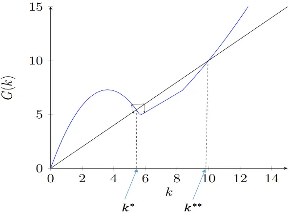
Proposition 7 (lucky growth). Let Assumption 4 be satisfied.
1. If G(x3)≤k∗∗, then kt ≤k∗∗ for any k0 ≤k∗∗.
2. If G(x3)> k∗∗, then we have: U(k∗∗)6=∅. In this case, limt→∞kt=∞ if and only
if k0 ∈U(k∗∗).
Moreover, if k0 ∈UT(k∗∗), then kt < k∗∗ for any t < T, kt> k∗∗ for any t > T.
Proof. See Appendix A.5.
The first point in Proposition7indicates that when the dynamics of capital are weak, then the economy never surpasses the middle-income trap.
Point 2 of Proposition 7 suggests that a poor country, receiving development aid and having strong dynamics of capital, may surpass the middle-income in a finite period and achieve growth in the long run. To understand better this point, let us consider
k0 ∈U0(k∗∗). When the dynamics of capital are strong (G(x3)> k∗∗), the stock of capital
at the next period will be high (thanks to development aid) and surpass the middle-income trap k∗∗ (i.e., k
1 = G(k0) > k∗∗), and then the recipient economy may reach
growth. However, in some cases, the economy needs more than one period to surpass the middle-income trap (for example, whenk0 ∈UT(k∗∗), the economy only surpassesk∗∗
after T periods).
21It is easy to see that the left hand side increases in ¯a, σ but decreasing in φ. It is increasing in α
Figure 5: Lucky growth vs. middle-income trap. Low curve corresponds to G(x3) < G(k∗∗),
with parameters β = 0.8, τ = 0.2;δ = 0.2, A = 0.4, σ = 1, αi = 0.7; ¯a = 12, b = 3, φ = 2.
High curve corresponds to G(x3) > G(k∗∗), with ¯a = 14, αi = 0.8, σ = 2, other parameters
unchanged.
Corollary 1. Let Assumption 4 be satisfied and assume that G(x3)> k∗∗. If the initial
capital k0 is close enough to x3, then limt→∞kt = ∞. However, if the initial capital k0
equals k∗ which is higher than x
3, we have kt =k∗, ∀t.
Figure 5 illustrates Corollary 1. If k0 = 5, then the economy grows in the long run;
however, if k0 = k∗ > 5, then kt = k∗ for any t. Corollary 1 suggests that a higher
initial capital does not necessarily help the economy to have more growth. Having growth without bounds, k0 must belong to U(k∗∗). For that reason, we use the term ”lucky
growth”, meaning that, with the same rule of aid, a poorer country may have growth but a richer country may not.
Pointing out this scenario is also a contribution of our paper to the literature on economic growth.
4.4
Discussion
sufficiently high. This result might justify a scaling-up of aid for countries suffering initial disadvantages which are not in favor of generating economic growth.
Concerning two intermediate circumstances (focusing on foreign aid or not), as we have shown in Section 4.2 and Section 4.3, their equilibrium outcomes are very different. On the one hand, under the intermediate circumstances 1 with domestic investment focus, k∗
is the only steady state and can be viewed as a poverty trap of the economy. The economy will collapse in the long run if and only if the initial capital of the country is lower than this trap. In this case, development aid may promote growth in the recipient country, but under the condition that the use of aid is efficient enough. On the other hand, under the intermediate circumstances 2 with foreign aid focus, there exists two steady states. The lower one k∗ can be interpreted as a middle-income trap. In this case, with foreign
aid, the economy never collapses, even if its initial capital is very low. However, it does not necessarily mean that the economy will grow in the long run. Instead, the outcomes are fragile. Indeed, it may converge to the middle-income trap or fluctuate around it. With some luck (strong dynamics of capital), the economy may benefit development aid to improve its public investment (including R&D) and thanks to this, it can surpass the poverty trap (i.e. the higher steady-state k∗∗) and get grow after a finite period. To sum
up, focusing on foreign aid would make the development process of the recipient country more complicated to predict.
4.5
Extensions
We now consider extensions of our framework to show the robustness of our results and insights. Assume now that aid flow is at = a(kt) instead of equation (1). The flow
of new technology depends on the tax revenue and the aid flow in the following way:
Ht = H τ kt, a(kt)
(instead of σBt). Assume that the TFP depends on new
tech-nologies: At = P(Ht). Consequently, the TFP has the following form instead of (4):
At=P
H τ kt, a(kt)
. The dynamics of capital (8a) becomes
kt+1 =G(kt)≡f(kt)kt, where f(kt)≡β
1−δ+PH τ kt, a(kt)
1 +τ (27)
We introduce natural assumptions on the functions a, P and H.
Assumption (a). The function a(·) :R+→R+ is continuous, concave, strictly
decreas-ing on [0,¯k] and differentiable on(0,¯k). a(0) = ¯a >0, a(k) = 0 ∀k≥k¯
Assumption (P). The function P(·) : R+ → R+ is continous, strictly increasing on
[b,∞)and differentiable on (b,∞). P(h)≥A >0∀h ≥0. P(h) = A if and only if h≤b
(A represents the autonomous productivity).
Assumption (H). The function H(·) : R2+ → R+ is differentiable, strictly concave,
strictly increasing in each component. The aid is not essential: H(x1,0) > 0 ∀x1 > 0.
Assume also that 1+τ
β +δ−1> A and H(∞,0)> hp where
hp ≡P−1
1 +τ
β +δ−1
. (28)
First, we study steady states. A steady state k >0 is determined by f(k) = 1, i.e.,
PH τ k, a(k)
= 1 +τ
Lemma 5. Let Assumptions (a), (P) and (H) be satisfied. There are at most 3 steady states.
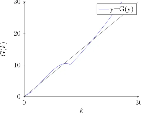
In the proof of Lemma 5 (see Appendix A.6), we provide a necessary and sufficient condition under which there are i(i=1,2,3) steady states. In particular, if H τ k, a(k)
=
σ(τ k)m 1 +α
i(¯a−φk)+ n
andP(h) = A(1 + (h−b)+), then there may be 3 steady states
as illustrated by the following figure.22
0 30
0 10 20 30
k
G
(
k
)
[image:23.628.195.434.200.392.2]y=G(y)
Figure 6: Existence of 3 steady-states.
Second, we look at the monotonicity of the policy function G(·).
Lemma 6. Let Assumptions (a), (P) and (H) be satisfied. If I′(x)≥0 ∀x∈[0,k¯), then
G′(x)>0 ∀x∈[0,k¯). By consequence, the function G is increasing on [0,∞).
Proof. See Appendix A.6.
Condition I′(x) ≥ 0, or equivalently τ H
1(τ x, a(x)) +a′(x)H2(τ x, a(x)) > 0, means
that the government always focuses on the domestic investment. With the specification (8b), conditionI′(x)≥0 becomes τ ≥α
iφ.
We now present our findings concerning the dynamics of capital (27). The following result is a generalized version of Proposition 2.
Proposition 8 (growth without bounds thanks to foreign aid). Let Assumptions (a), (P) and (H) be satisfied. If min H(τk,¯ 0), H(0,¯a)
> hp, then two statements in Proposition 2 hold.
Proof. See Appendix A.6.
Notice that condition in Proposition 8 is more likely to be satisfied if : (1) the fixed cost b is low and/or the autonomous productivity A is high (because hp is increasing in
b and decreasing in A); or/and (2) the aid rule is generous in the sense that ¯a is high and/or φ is low (because min H(τk,¯ 0), H(0,¯a)
is increasing in ¯a and decreasing in φ). We now extend Proposition 3 as follows:
22Parameters are: β = 0.8;τ = 0.2;δ = 0.2;A= 0.4;σ= 2.5;α
Proposition 9. (growth or collapse? The role of aid.) Let Assumptions (a), (P) and (H) be satisfied. If x 1−δ+P(I(x))
is increasing on [0,k¯], then G is increasing on [0,∞). In this case, three statements in Proposition 3 hold.
According to this result and Lemma 6, we have that: if I′(x) = τ H
1(τ x, a(x)) +
a′(x)H
2(τ x, a(x)) > 0, meaning that the government always focuses on the domestic
investment, then three statements in Proposition 3 hold.
We now present results in the case where the policy function may not be increasing. Denote k∗∗ the unique solution (if it exists) of the equation H(τ k,0) = h
p. We firstly
look at the economic growth in an economy having a high initial capital.
Proposition 10 (high initial capital). Let Assumptions (a), (P) and (H) be satisfied and
H(τ¯k,0)< hp. We have that: (1)k∗∗is the highest steady state; and (2) for anyk0 > k∗∗,
the sequence (kt) increases and the economy grows without bounds.
Proof. See Appendix A.6.
We next look at countries having a low initial capital level. The following result generalizes Proposition 4.
Proposition 11 (low initial capital). Let Assumptions (a), (P) and (H) be satisfied.
1. Assume that β1−δ+P1+(Hτ(0,¯a)) > 1. If the initial capital stock k0 is low enough, then
the capital stock at the next period will be higher than k0: k1 > k0.
2. Assume that β1−δ+P1+(Hτ(0,¯a)) < 1. If the initial capital stock k0 is low enough, then
limt→∞kt= 0.
Proof. See Appendix A.6.
Different from Proposition 4, we also provide a condition under which the economy collapses. This is illustrated by Figure 6where we see that, if the initial capital k0 is less
than the lowest steady state, then kt converges to zero.
As Proposition 7, we can prove the following result concerning the dynamics of economies having middle initial capital.
Proposition 12 (middle initial capital). Let Assumptions (a), (P), (H) be satisfied and
H(τ¯k,0)< hp.
1. If maxx∈[0,k∗∗]G(x)≤k∗∗, then kt ≤k∗∗ for any k0 ≤k∗∗.
2. If maxx∈[0,k∗∗]G(x)> k∗∗, then we have: U(k∗∗)defined by (26a, 26b) is not empty, and limt→∞kt=∞ ∀k0 ∈U(k∗∗). Consequently, aid flowat= 0 for t high enough.
We end this section by mentioning two remarks.
Remark 4 (on the essentiality of aid). Let Assumption 1 be satisfied. We can prove that, if the aid is essential in the sense that H(x1,0) ≤ b ∀x1 > 0, then kt is bounded
from above.23 This leads to an interesting implication: if the foreign aid is essential for
the realization of the public investment in the recipient country whose autonomous TFP is not high, then this country never grows.
23It suffices to prove thatk
t+1< ktifkt>k¯. Indeed, ifk >k¯, thena(k) = 0 and henceH(τ k, a(k)) =
H(τ k,0) ≤ b. This implies that P(H(τ k, a(k)) = A. By consequence, f(k) = β(11+−δτ+A) < 1. So,
Remark 5 (link to Dalgaard (2008)). If we consider a particular case with a full depre-ciation of capital (δ = 1), no fixed cost (b = 0), no capital tax (τ = 0), and the rule of aid flows is given by at=θktλ where θ >0, λ <0 as in Dalgaard (2008), the dynamics of
capital will be
kt+1 =βAσαiθktλ+1 (30)
Then, we recover a dynamic system similar to that in Dalgaard (2008). The transitional dynamics of capital stock in (30) are much simpler than (8a) or (27) in our framework. In Dalgaard (2008) or in (30), the characteristics of the transitional path are determined by λ(the degree of inequality aversion on the part of the donor) while in our model they depend on all parameters. In particular, the model in Dalgaard (2008) has at most one steady state while ours may have two, even three.
5
Foreign aid in a centralized economy
We have so far focused on the outcomes in competitive equilibrium. In this section, we investigate the effects of foreign aid in a centralized economy. The social planner maximizes the intertemporal utility P+∞
t=0 βtu(ct) by choosing consumption (ct), physical
capital (kt) and tax (Tt) subject to sequential constraints: ct+kt+1+Tt≤F(kt, Tt−1, at),
∀t ≥ 1 where w0 ≡ F(k0, T−1, a0) is given and the aid flow at = a(kt) is a decreasing
function of kt. We assume that F(kt, Tt−1, at) = AtF0(kt) where F0 is the autonomous
production function and At=P
H Tt−1, a(kt)
is the TFP at date tdepending on new technologies as in Section 4.5.
Denote St ≡ kt+1 +Tt, kt+1 = θSt, Tt = (1−θ)St where θ ∈ [θ1, θ2] ⊆ [0,1], where
parameters θ1, θ2 represent other potential constraints of the government, which we do
not model here. The problem of the social planner can be rewritten as follows
(CP1) : max(ct,St)+
∞
t=0
P+∞ t=0 β
tu(c
t) (31a)
s.t: ct+St≤q(St−1) (31b)
whereq(x)≡maxθ∈[θ1,θ2]Q(x, θ), and Q(x, θ)≡F0(θx)P
H (1−θ)x, a(θx) (31c)
and q(s−1) ≡ w0 > 0 is given and the utility function u satisfies standard conditions as
required in Le Van and Dana(2003), Kamihigashi and Roy (2007).24
In particular, if there is no aid andF0(x) =xαd,H(x) = Aexαe,P(x) =A+a(x−x¯)+,
we recover the model in Section 3.1 in Bruno et al. (2009).
Observe that the outcomes (consumption, physical capital, and production) of the social planner’s problem are different from those in the decentralized economy. There are two reasons: (1) the presence of externalities in the production function, and (2) the tax rate Tt/St is endogenous in the central planner’s problem (CP1) while it is exogenous in
the maximization problem of the household (Pc).
If the functionQ(x, θ) is increasing inx, then so is the function q(x). However, theses two functions may not be increasing. Moreover, they may not be concave and there are
24Precisely, we assume that (1)uis inC1, strictly increasing and concave andu′(0) =∞, (2) for every
S >0, there exists a feasible path (ct, St) fromSsuch thatP∞t=0β
tu(ct)>−∞and (3) for everyS >0, we have P∞
t=0β
two thresholds in the function Q(x, θ). By consequence, providing a full global analysis of the solution of the optimal growth problem (CP1) is a challenge. However, some clear-cut points can be obtained. As in Section 2 and for the sake of tractability, we assume that
Q(x, θ)≡θx1−δ+Ah1 +
σ(1−θ)x+σαi(¯a−φθx)+−b +i
. (32)
Even under this specification, the solution of the problem (CP1) is not explicit as that in Section 2.4. In order to study the properties of optimal paths, we have to understand when q(x) and Q(x, θ) are increasing or decreasing. Similar to Lemmas 1and 2, we can identify conditions under which the function Q(x, θ) is increasing inx or not.
Lemma 7 (monotonicity of Q(x, θ) in x). Denote
y1 ≡
¯
a
φθ, y2 =
σαi¯a−b
σ(θ(1 +αiφ)−1)
, y3 ≡
1−δ+A(1 +σαi¯a−b)
2Aσ θ(1 +αiφ)−1
(33)
where θ is given such that y1, y2, y3 are well defined.
We have that Q(x, θ) is increasing in x on [y1,∞). Moreover,
1. If 1−θ(1 +αiφ)≥0, then Q(x, θ) is increasing in x.
2. If θ(1 +αiφ)−1>0 and σαia¯−b≤0, then Q(x, θ) is increasing in x.
3. If θ(1 +αiφ)−1 > 0 and σαia¯−b > 0. In this case, y2, y3 > 0, and Q(x, θ) is
increasing in x on [y2,∞)
(a) If y3 ≥min(y1, y2), then Q(x, θ) is increasing in x.
(b) Ify3 < min(y1, y2), thenQ(x, θ)is increasing on[0, y3], decreasing on[y3,min(y1, y2)],
and increasing on [min(y1, y2),∞).
When θ(1 +αiφ)−1>0 andσαi¯a−b >0, we observe that
y3 ≥y1 ⇔
1
θ >1 +αiφ−φ
1−δ+A(1 +σαi¯a−b)
2Aσ¯a while y3 ≥y2 ⇔1−δ+A≥A(σαia¯−b).
By consequence, we have the following result.
Corollary 2. Given θ ∈ [θ1, θ2]. The function Q(·, θ) is increasing on [0,∞) if one of
the following conditions holds.
1. θ2(1 +αiφ)≤1.
2. θ1(1 +αiφ)>1 and σαi¯a≤b.
3. θ1(1 +αiφ)>1, σαi¯a > b, and 1−δ+A≥A(σαi¯a−b).
4. θ1(1 +αiφ)>1, σαi¯a > b, and θ12 >1 +αiφ−φ1−δ+A(1+σα
i¯a−b)
2Aσa¯ .
Interpretations: condition θ2(1 +αiφ) ≤ 1 is equivalent to 1 −θ2 ≥ 1+αiαφiφ which
ensures that the government focuses on the investment in new technology/innovation (because Tt/St = 1−θ ≥1−θ2). Conditions 2 and 3 mean that the government focuses
on the physical capital (θ1 is high) and the aid is not very generous (φ is high). Under
condition 4, the government takes care of both the physical capital (θ1 is high) and the
investment in new technology/innovation (θ2 is not high).
Proposition 13. (1) Under conditions in Corollary 2, the function q(x) is increasing, and then the optimal capital path (kt) is monotonic and converges.
(2) If θ1 = θ2 = θ, θ(1 +αiφ) ≤ 1, σαi¯a > b and βθ 1−δ+A 1 +σαi¯a−b)
>1, then every optimal capital path motonically goes to infinity and aid flow at becomes zero
when t is high enough.
Proof. See Appendix A.7.
In Proposition 13, since the function q(x) is increasing, we can apply the optimal growth theory (see Le Van and Dana(2003),Kamihigashi and Roy (2007) among others) to study properties (convergence, boundedness, growth, ...) of optimal capital paths. Conditions in the second statement of Proposition 13 mean that the government focuses on the investment in new technology/innovation, the level of efficiency σ is high, and the aid is generous enough. Under these conditions, the economy obtains growth in the long run whatever the level of initial output. The insight is similar to that of Proposition 2
even though the approches and proofs are different. Proposition 2’s second part is also in line with Proposition 3 of Bruno et al.(2009). Our added value is to introduce foreign aid and study its effects.
However, the functionsq(x) andQ(x, θ) may be decreasing inx. According to Lemma
7, the function Q(x, θ) is not increasing in x only if σαi¯a > b and θ2(1 +αiφ)−1 > 0.
In such a case, we obtain the following result showing the role of the TFP A and of the efficiency σ as well as of the aid rule (¯a, φ).
Proposition 14. We now assume that σαia > b¯ and θ2(1 +αiφ)−1>0.
Assume that the initial output of the economy w0 is low in the sense that 2σ(1 +
αiφ)w0 < σαi¯a−b and 4αiφσw0 < σαi¯a−b.
1. If βθ2
1−δ+A+ A
2(σαi¯a−b)
> 1, then c1 > c0 for any optimal path, and by
consequence no optimal path converges to zero.
2. If 1−δ+A(1 +σαia¯−b)< 1, then the economy collapses (St and ct converge to
zero).
Proof. See Appendix A.7.
The insight of po