Intertemporal Consumption with Risk: A Revealed Preference Analysis

Munich Personal RePEc Archive

Intertemporal Consumption with Risk:

A Revealed Preference Analysis

Lanier, Joshua and Miao, Bin and Quah, John and Zhong,

Songfa

Oxford University, Shanghai University of Finance and Economics,

Johns Hopkins University, National University of Singapore

1 February 2018

Online at

https://mpra.ub.uni-muenchen.de/86263/

Intertemporal Consumption with Risk:

A Revealed Preference Analysis

Joshua Lanier, Bin Miao, John K.-H. Quah, Songfa Zhong

February 2018

[Preliminary and Incomplete]

Abstract

This paper presents a nonparametric, revealed preference analysis of intertemporal consumption with risk. In an experimental setting, subjects allocate tokens over four commodities, consisting of consumption in two contingent states and at two time periods, subject to different budget constraints. With this data, one could test, using Afriat’s Theorem and its generalizations, whether a subject’s choices are consistent with utility maximization, and also utility maximization with various additional properties on the utility function. Our results broadly support a model where subjects maximize a utility function that is weakly separable across states but there is little support for weak separability across time. Our result sheds light on the source of the failure of the discounted expected utility model.

Keywords: risk preference, time preference, revealed preference, budgetary choice, Afriat’s Theorem, experiment

1

Introduction

Many important economic decisions involve agents choosing among alternatives that differ in both their risk and time properties. The canonical way of representing preferences in this context is to combine the expected utility and discounted utility models into what is known as the discounted expected utility (DEU) model, which evaluates the utility of a contingent consumption plan (ec1,ec2,ec3, ...) as

(1) X

t

δtE[u(ect)],

where ect is the random consumption in period t and δt is the corresponding discount factor.

With (additive) separability across both time periods and states, DEU has the great advantage of being a simple and tractable model which can deliver sharp conclusions in different applied contexts. However, this simplicity also means that the model cannot distinguish between an agent’s attitude towards risk and his attitude towards intertemporal consumption. For this reason and others, alternative models have been proposed, which dispenses with separability either across states or across time (e.g., Kreps and Porteus, 1978; Selden, 1978; Epstein and Zin, 1989; Chew and Epstein,1990; and Halevy, 2008; see Section 1.1 for a more detailed discussion). Notably, some of these models have been shown to capture a broader domain of phenomena, such as the equity premium puzzle (Epstein and Zin, 1991).

In this paper, we design an experiment which will allow us to find out, using purely nonparametric methods, the source of the departure from the DEU model. In our experiment, subjects allocate experimental tokens to four commodities, which pay out in two states s1

and s2 and two time periods t1 and t2, as follows:

t1 t2

s1 c11 c12

s2 c21 c22

The two states s1 and s2 are set to be equiprobable, while t1 and t2 are one week later and

nine weeks later respectively. Subjects allocate 100 tokens by choosingc= (c11, c12, c21, c22)

subject to the budget constraint

(2) p11c11+p12c12+p21c21+p22c22≤100.

We present subjects with different budget sets by varying the price vectorp= (p11, p12, p21, p22),

ours is the first experiment in which subjects choose among affordable alternatives where payoffs vary in two dimensions, i.e., in both state and time.

From each subject, we obtain a dataset with 41 observations, with each each observation

i consisting of a price vector pi _{= (p}

11, p12, p21, p22) and the corresponding choice ci =

(c11, c12, c21, c22) made by the subject at that price vector. Throughout the paper, we apply

(nonparametric) revealed preference methods to test alternative hypotheses on a subject’s utility function U defined on the contingent consumption plan c∈R4

+. At the most general,

we ask whether the subject is maximizing some well-behaved (i.e., strictly increasing and continuous) utility function U. In other words, we ask whether there exists a function U

such that the subject is choosing optimally given his budget; formally, at every observation i, we require U(ci_{)≥U(c) for all csatisfying the budget constraint (2), with p=p}i_{. Afriat’s}

Theorem (see Afriat (1967) and Varian (1982)) establishes that a data set O ={(pi_{, c}i_)}41

i=1

is consistent with this utility-maximization hypothesis if and only if it obeys GARP (the generalized axiom of revealed preference), a property which is computationally straightforward to check.

If the subject is maximizing discounted expected utility, then (with equiprobable states)

(3) U(c11, c12, c21, c22) =

1

2u(c11) + 1

2δu(c12) + 1

2u(c21) + 1

2δu(c22).

for some increasing function u andδ ∈(0,1). DEU is a special case of a utility function that is weakly separable across states, which has the general form

U(c11, c12, c21, c22) = F(υ(c11, c12),eυ(c21, c22)),

where υ (˜υ) is the sub-utility function over consumption streams in state 1 (state 2) and

F aggregates over the two sub-utilities. (In the DEU case, υ(c11, c12) = u(c11) +δu(c12),

˜

υ(c21, c22) = u(c11) +δu(c12) and F is the simple average between these two sub-utilities.)

The DEU form is also a special case of a utility function that is weakly separable across time, which has the general form

U(c11, c12, c21, c22) =G(ω(c11, c21),ωe(c12, c22)).

In this case, ω (˜ω) is a sub-utility function over state-contingent consumption at date 1 (date 2) and the two sub-utilites are aggregated by the function G.

If a subject is a DEU maximizer, his datasetO = {(pi_{, c}i_)}41

i=1 will obey properties beyond

for state 2. In other words, ci s1 = (c

i

11, ci12) must be optimal at price pis1 = (p

i

11, pi12) in the

sense thatυ(ci

s1)≥υ(c11, c12) for all (c11, c12) obeying (p

i

11, pi12)·(c11, c12)≤(pi11, pi12)·(ci11, ci12).

Therefore, if O is collected from a DEU maximizer, or more generally from a subject with a utility function weakly separable across states, the spliced data setsOs1 ={(p

i s1, c

i s1)}

41

i=1 and

Os2 ={(p

i s2, c

i s2)}

41

i=1 will both obey GARP.

By a similar logic, if a data set is collected from a DEU maximizer or more generally from an agent with a utility function that is weakly separable across time, then GARP holds if O

is spliced along the time dimension, i.e., Ot₁ = {(pit1, c

i t1)}

41

i=1 and Ot2 ={(p

i t2, c

i t2)}

41

i=1 will

both obey GARP, where pi t1 = (p

i

11, pi21) and cit1 = (c

i

11, ci21).

When we test the data for these properties, we find that, in general, O obeys GARP and so does Os1 and Os2, but that is not true of Ot1 and Ot2. In other words, there is general

support for utility maximization broadly defined and also for the existence of sub-utility functions defined on consumption streams, but there is weak support for sub-utility functions defined on contingent consumption. Furthermore, there is evidence that the sub-utility function on consumption streams is the same in both states, i.e., υ = ˜υ and also that this sub-utlity function exhibits impatience, i.e., one could find a rationalization of Os1 such

that υ(x, y)≥ υ(y, x) wheneverx ≥y. Testing for rationalizability with a utility function exhibiting impatience requires a strengthening of the GARP property (see Nishimura, Ok, and Quah (2017)).

These results suggest that, for most subjects, a utility function that is weakly across states but not necessarily across time captures their behavior well. Indeed, there is a generalization of Afriat’s thoerem to test for rationalizabitliy with a weakly separable utility function (see Quah (2014)). Using this test, we find that 26% of the subjects satisfy both state and time separability (approximately), 50% of the subjects satisfy state separability but not time separability, 4% of the subjects satisfy time separability but not state separability, 11% of the subjects satisfy neither state separability nor time separability, the rest of 10% fail the overall GARP test and are not consistent with utility-maximization for the most general utility functionU.

1.1

Related Literature

plan the uncertainty resolves at period 1 and in the other at period 2. In relaxing time neutrality, Kreps and Porteus (1978) obtains a recursive expected utility representation that is essentially time non-separable. Selden (1978) and Epstein and Zin (1989) focus instead on the non-distinction between risk preference and time preference in the DEU model. To illustrate, notice that DEU reduces to expected utility E[u(_ec)] for degenerate contingent consumption

e

c, and to discounted utility Pδtu(ct) for a deterministic consumption stream (c1, c2, c3, ...).

Therefore, the same utility index u captures both the attitude towards risk and the attitude towards intertemporal substitution. The utility forms proposed in both Selden (1978) and Epstein and Zin (1978) disentangle risk preference from time preference, but Selden (1978) relaxes state separability while Epstein and Zin (1989) relaxes time separability. Follow-up models, including Chew and Epstein (1990) and Halevy (2008), attempt to distinguish risk preference from time preference by incorporating non-expected utility.

A number of recent experimental studies investigate various aspects of attitude towards intertemporal risks. Andreoni and Sprenger (2012a) propose an experimental design termed Convex Time Budget (CTB) to elicit time preference. In this experiment, subjects make allocation decisions between sooner and later payment. Andreoni and Sprenger (2012a) find that the utility index for time preference elicited using CTB is distinct from the utility index for risk elicited using price list. Relatedly, Abdellaoui et al. (2013) introduce a method to measure utility functions for risk preference and time preference separately, and find that the utility function under risk is more concave than the utility function over time. In another paper, Andreoni and Sprenger (2012b) consider CTB under a risky environment, in which there is a 50 percent chance of receiving the earlier payment and, independently, another 50 percent chance of receiving the later payment; they find that subjects are more responsive to changes of interest rate in the risky environment than under certainty. Based on these experimental results, Andreoni and Sprenger (2012a, b) conclude that risk preference is distinct from time preference. Epper and Fehr-Duda (2015) show theoretically that rank-dependent probability weighting (Halevy, 2008) can account for the key findings in Andreoni and Sprenger (2012b). Miao and Zhong (2015) also experimentally investigate intertemporal decision making and find support for a separation between attitudes towards risk and attitudes towards intertemporal substitution; their findings are broadly consistent with the models of Epstein and Zin (1989), Chew and Epstein (1990), and Halevy (2008). These experimental studies focus on the distinction between the utility index for risk aversion and intertemporal substitution, but they do not directly test for the separability of subjects’ utility function across states and across time. The current study provides the first experimental test examining this issue.

experimental literature where budgetary choice decisions are employed to study preferences. Other instances include Andreoni and Miller (2001) and Fisman, Markovits and Kariv (2007), which study social preferences by considering modified dictator games in which the subjects allocate tokens between herself and anonymous recipients, with the value of each token varying across observations. Choi et al. (2007) study risk preferences by having subjects make portfolio decisions involving contingent consumption. Our study could be thought of as an extension of the Choi et al. (2007) experiment to one where risk and time preferences are studied in conjunction.

Whenever budgetary decisions are analysed, it is commonplace to appeal to Afriat’s Theorem to study rationalizability or approximate rationalizability, the latter through the use of the critical cost efficiency index (Afriat, 1974). For example, Choi et al. (2015) find, in a large-scale experiment with household subjects, that the level of choice consistency with utility maximization, as measured by this index, is positively correlated to wealth. It is less common to go beyond Afriat’s Theorem to use other revealed preference tests to evaluate the consistency of decision making with more specific models of utility maximization; examples of this include Polisson, Quah, and Renou (2015) for risk preference and Saito, Echenique and Imai (2015) for time preference. The use of revealed preferences tests beyond GARP is a feature of this paper.

1.2

Organization of the paper

Section 2 presents the experimental design. Since results in revealed preference analysis are used extensively in the paper, these are explained in some detail in Section 3. The results of the experiment are report in Section 4 and Section 5 concludes. There is also an Appendix with more detailed results.

2

Experiment Design

This section describes the design of our experiment, in which subjects make allocation decisions under different budget constraints. Specifically, we provide subjects with a budget of 100 experimental tokens which they can allocate over four date and state contingent commodities. A typical consumption bundle can be written as c= (c11, c12, c21, c22) where cst

refers to consumption in states at time t. The two states, determined by a coin toss, are of equal probability; and the two time points are one week later and 9 weeks later.

The price vectorp= (p11, p12, p21, p22) is obtained by having the price for each commodity

1. This gives rise to 96 distinct price vectors. We randomly select 41 price vectors for each subject with one of them fixed to be the benchmark vector (1,1,1,1).

At the end of the experiment, each subject is paid according to one randomly selected decision task by tossing dice according to the Random Incentive Mechanism (RIM).1

Subjects are informed to treat each decision as if it were the sole decision determining their payments. To control for preference for the timing of uncertainty resolution, all uncertainty is resolved at the end of the experiment. Once the decision task is selected and the state is realized, each subject is paid with an exchange rate of SGD 0.2 (about USD 0.15) per experimental token. To increase the credibility of payment, subjects are paid with post-dated checks that will not be honored by the local bank when presented prior to the date indicated. To further control for the potential difference in transaction cost at different time points (Andreoni and Sprenger, 2012a), subjects receive a minimum participation fee of SGD 12 (with SGD 6 for each payday). Experimental earnings are added to these minimum payments.

We note that the experiment in this study is based on monetary reward while in most models utility is derived from actual consumption. Reuben, Sapienza, and Zingales (2010) elicit discount factors for both monetary rewards and primary rewards of chocolate and find a positive and statistically significant relation between discount rates elicited using monetary and primary rewards. The observed correlation suggests that measurement through monetary reward might be ecologically valid. Augenblick, Niederle, and Sprenger (2013) study time preference over effort and show that the incentive for smoothing is higher for effort than for monetary reward. Readers can refer to Halevy (2014) for insightful discussions on the validity of using cash payment to elicit time preference. Notwithstanding these caveats, we posit that our overall approach would be applicable to the settings with actual consumptions.

A total of 103 undergraduate students are recruited as participants through an adver-tisement posted in the Integrated Virtual Learning Environment at the National University of Singapore. The experiment is conducted at the laboratory of the Center for Behavioral Economics at the National University of Singapore. Conducted by two of the authors and a research assistant, the experiment consists of four sessions with 20 to 30 subjects in each session. After the subjects arrive at the experiment venue, they are given the consent form approved by the Institutional Review Board of the National University of Singapore. Following that, general instructions are read aloud to the subjects, and several examples are demonstrated to them before they started making their decisions. The experimental instructions follow closely those in Andreoni and Sprenger (2012b) (See Appendix C for the Experimental Instructions). Most of our subjects complete the tasks within 30 minutes. At the end of the experiment, they approach the experimenters one by one, toss the dice and

1

receive payments in post-dated checks based on their choice. On average, the subjects are paid SGD 22.

3

Revealed Preference Analysis

In Section 3.1 we describe and explain the basic GARP condition that characterizes rational-izability with a well-behaved utility function. In Section 3.2 we consider further properties which we may require of a utility function rationalizing a dataset, and show how the GARP condition could be modified to check for rationalizability with utility functions having those properties.

3.1

GARP

We denote bypi _{= (p}i

11, pi12, pi21, pi22) the price vector faced by the subject in decision problem

i, and by ci _{= (c}i

11, ci12, ci21, ci22) the bundle chosen by the subject. Thus the collection of a

subject’s decisions for allI decision problems can be written as

O=(p1, c1), . . . ,(pI, cI) .

We shall refer to such a collection as a dataset. A utility function U :R4

+ →R rationalizes

the dataset O if, at each observation i∈I,2

U(ci)≥U(c) for all c∈R4+ s.t. p

i_·ci _≥pi_·c.

This condition states that if a subject can afford cwhen choosingci_{,then it must be the case}

that the utility derived from ci _{is weakly higher than that derived from c.}

We refer to a utility function (or more generally any function defined on a subset of the Euclidean space) as well-behaved if it is continuous and strictly increasing. Afriat’s Theorem (see Afriat (1967) and Varian (1982)) provides a necessary and sufficient condition under which a dataset can be rationalized by a well-behaved utility function. We shall now describe that test.

Let C ={ci}i∈I be the set of bundles chosen by the subject at some observation i. Given

a datasetO, if a subject chooses ci _{when some c}j _{in C is affordable (i.e., p}i_·ci _≥pi_·cj_{), then}

we say that ci _{is directly revealed preferred to c}j _{and denote it by c}i _%∗ _cj_{. If c}j _{is strictly}

cheaper than ci _(pi_·ci _{> p}i_·cj_{), then we say that c}i _{isdirectly strictly revealed preferred to c}j

and denote it by ci _≻∗ _cj_{. Lastly, let therevealed preferred relation be the transitive closure}

2

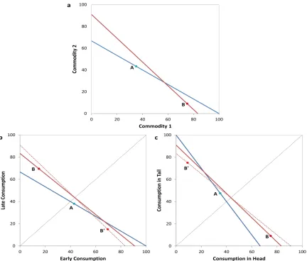
Figure 1: Illustration of violations of GARP, Impatience and Symmetry. Fig 1.a depicts a violation of GARP, sinceA is revealed strictly preferred toB and B is revealed strictly preferred toA. GARP is not violated in Fig 1.b; however it is not consistent with optimization with an impatient utility function. B is revealed strictly preferred to Aand A is also revealed strictly preferred toB under the impatience assumption, since B′ _{is contained in the budget set whenA is chosen and the impatient}

subject must prefer B′ _{to B. In Fig 1.c, GARP is not violated, but the data is not compatible with}

maximization of a symmetric utility function. B is revealed preferred toA and, under symmetry A

is revealed preferred to B (because A is revealed preferred to B′_).

of %∗_{, denoted as %}∗∗_.3

A dataset O satisfies the generalized axiom of revealed preference

(GARP) if the following holds:

(4) for all ci and cj, ci %∗∗

cj impliescj ⊁∗

ci.

Figure 1.a depicts a violation of GARP involving two observations. It is not difficult to show

3

In detail,ci_%∗∗ _cj _{if we can findi}

that any dataset that can be rationalized by a well-behaved utility function (indeed, by any locally nonsatiated preference) must satisfy GARP; the substantive part of Afriat’s Theorem establishes that GARP is also sufficient for a dataset to be rationalized by a well-behaved utility function.

GARP tests provide 0/1 results, i.e., a subject is either consistent or inconsistent with maximizing a specific utility function. However, a subject may behave roughly in accordance with utility maximization but for some reason such as inattention and measurement error, the subject does not choose the optimal bundle on all occasions. A popular approach to measure departures from rationality to use thecritical cost efficiency index(CCEI) developed in Afriat (1972). This index, which ranges from 0 to 1, is a measure of the efficiency with which a subject allocates his budget. Formally, a subject has a CCEI of e∈[0,1] if e is the largest number such that there is a well-behaved utility function U with

(5) U(ci)≥U(c) for all c∈R4+ s.t. p

i_·ci _{≥e p}i_{·c, for all i∈I.}

A CCEI of 1 indicates that a subject is perfectly utility-maximizing. A CCEI less than 1, say 0.95, indicates that there is a well-behaved utility function that approximately rationalizes the data in the sense that there is a utility function for which the chosen bundle ci _(at

every observation i) is preferred to any bundle that is more than 5% cheaper than ci _{(at the}

prevailing price vector pi_).

Approximate rationalizability at some coefficient e (in the sense given by (5)) can be tested using a modified version of GARP, in which the revealed preference relation %∗

e is

defined as follows: ci %∗

e cj if pi·ci ≥e pi·cj. In an analogous way, one could define ≻

∗

e, the

transitive closure %∗∗

e and the no-cycling condition (4). Such a condition is necessary and

sufficient for rationalizability at that coefficient (see Afriat (1972)).

3.2

More revealed preference tests

The basic GARP test could be extended in various ways to test for more stringent conditions on the rationalizing utility function. We confine our discussion here to those properties which must be satisfied by any subject who maximizes a discounted expected utility function. It follows that a rejection of any of these properties implies a rejection of the discounted expected utility model.

Property 1: State Separability. A utility function U satisfies state separability if there are well-behaved functions F :R2

→R, υ,υ_e:R2

+ →R, such that

State separability implies that the consumption stream in one state can be ordered inde-pendently of what is obtained in the other state. Therefore, if two bundles give the same consumption stream in (for example) state 2, then altering that stream will not change the preferred bundle, i.e.,

t1 t2

s1 x y

s2 z w

≻

t1 t2

s1 x′ y′

s2 z w

⇒

t1 t2

s1 x y

s2 z′ w′

≻

t1 t2

s1 x′ y′

s2 z′ w′

Property 2: Time Separability. A utility function U satisfies time separability if there are well-behaved functions G:R2

→R, ω,_eω:R2

+ →R, such that

(7) U(c11, c12, c21, c22) =G(ω(c11, c21),ωe(c12, c22)).

In this case, the ranking over two bundles with the same contingent consumption at (say) date 1 will not be altered if the date 1 contingent consumption is changed, i.e.,

t1 t2

s1 x y

s2 z w

≻

t1 t2

s1 x y′

s2 z w′

⇒

t1 t2

s1 x′ y

s2 z′ w

≻

t1 t2

s1 x′ y′

s2 z′ w′

For a data set to be rationalizable by a utility function that is weakly separable across states, it is clear that GARP should be satisfied byO, and it should also be satisfied when the data is restricted to each state; in other words, Os₁ =

pi s1, c

i

s1 i∈I (where p i s1 = (p

i

11, p

i

12)

and ci s1 = (c

i

11, ci12)) and Os2 =

pi s2, c

i

s2 i∈I must both obey GARP. However, these three

conditions together are notsufficient to guarantee weak separability.

Necessary and sufficient conditions for weak separability can be found in Quah (2014). We shall now describe that test, focusing on the case of state separability. First, we must find a complete and transitive relation,%s1 onCs1 ={c

i

s1}i∈I that extends the revealed preference

and revealed strict preference relations on Cs1, 4

and another complete and transitive relation on Cs2 ={c

i

s₂}i∈I that extends the revealed preference and revealed strict preference relations

Cs2. Based on %s1 and %s2, we then construct a revealed preference relation onC such that

ci _{is revealed preferred to c}j _{if there exist c}k

s1 ∈ Cs1 and c

ℓ

s2 ∈ Cs2 obeying the following

conditions: (i) (pi s1, p

i s2)·(c

i s1, c

i

s2)≥(p

i s1, p

i s2)·(c

k s1, c

ℓ

s2); (ii) c

k

s1 %s1 c

j

s1; and (iii) c

ℓ

s2 %s2 c

j s2.

We say that ci _{is revealed strictly preferred to c}j _{if either the inequality in (i) is strict, or}

either of the preferences in (ii) and (iii) are strict. Quah (2014) shows that if %s1 and%s2

could be found so that the resulting revealed relations admit no cycles in the sense of (4),

4

The complete and transitive relation%s₁ extendsthe revealed preference relations ifci

s1 %s1 (≻s1)c

j s1 if

then the data is rationalizable by a utility function that is weakly separable across states.5

(It is clear that this condition is also necessary.)

If a subject has a utility function that is weakly separable across states, then it would be natural to expect the sub-utility functions (which are defined on consumption streams over time) to exhibit impatience. This means that given a larger quantityxand a smaller quantity

y, an impatient subject would prefer the larger quantity early and the smaller quantity later.

Property 3: Impatience. x≥y implies υ(x, y)≥υ(y, x), and υe(x, y)≥υe(y, x).

Similar to the test for weak separability, the test for this property involves strengthening the revealed preference conditions and then testing for the absence of cycles. We focus our discussion on consumption streams in state 1. For ci

s1 and c

j

s2 in Cs1, we say that

ci s1 = (c

i

11, ci12) is revealed preferred to cjs1 = (c

j

11, c

j

12) if either (i) pis1 ·c

i s1 ≥ p

i s1 ·c

j

s1 or (ii)

pi s1 ·c

i s1 ≥p

i s1 ·(c

j

12, c

j

11) and c

j

12 > c

j

11. In addition, cis1 is revealed strictly preferred toc

j s1 if

either (ii) holds or the inequality in (i) is strict. With these modified definitions of revealed preference, it is straightforward to check that the no-cycling condition (4) is necessary for rationalization by a well-behaved utility functionυ exhibiting impatience; furthermore, this condition is also sufficient for rationalization by a utility function with these properties (see Nishimura, Ok, and Quah (2017)). Figure 1.b depicts a dataset with two observations that obeys GARP but cannot be rationalized with an impatient utility function.

In the case where there is weak separability across time, the sub-utility functions ought to be symmetric since the two states are equiprobable in our experiment.

Property 4: Symmetry. ω(x, y) = ω(y, x) and ωe(x, y) = ωe(y, x), for any x, y∈R+.

To explain the test for this property, we focus our discussion on contingent consumption at date 1. Let Ct₁ = {cit1}i∈I, where c

i t1 = (c

i

11, ci21). For cit1 and c

j

t1 in Ct1, we define c

i t1 as

revealed preferred to cj_t

1 if either (i) p

i t1 ·c

i t1 ≥ p

i t1 ·c

j

t1 or (ii) p

i t1 ·c

i t1 ≥ p

i t1 ·(c

j

21, c

j

11). In

addition, ci

t1 is revealed strictly preferred toc

j

t1 if either (i) or (ii) holds with strict inequality.

With these modified definitions of revealed preference, it is straightforward to check that the no-cycling condition (4) is necessary for rationalization by a well-behaved and symmetric utility function ω; less obviously, this condition is also sufficient (see Nishimura, Ok, and Quah (2017)). Figure 1.c gives an example of a dataset with two observations that obeys GARP but is not rationalizable with a symmetric utility function.

Lastly, it would be natural to hypothesize that any sub-utility over consumption streams is state independent, in the sense that υ = υe, and that any sub-utility over contingent consumption would be time-invariant, in the sense that ω =ωe,

5

Property 5: State-Independent Time Preference. υ =υ_e.

Property 6: Time-Invariant Risk Preference. ω =ω.e

Property 5 can be tested by pooling Os₁ and Os₂ into a single data set and then

checking if it is rationalizable, either with a well-behaved utility function or a well-behaved and impatient utility function. Similarly, time-invariance can be tested by pooling Ot1 and

Ot2.

Lastly, we should mention that even though throughout this subsection we have confined our discussion to testing for exact rationalizability, it is possible to modify these tests to measure the critical cost efficiency index when exact rationalizability fails. The approach is broadly the same as that (described at the end of Section 3.1) for the standard GARP test.

4

Results

4.1

Aggregate Behavior

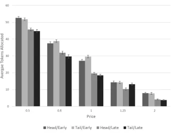
This subsection provides a brief summary of aggregate behavior. Figure 2 plots the average allocation of tokens for each of the four commodities under each price.6

Two patterns arise. First, the average allocation is lower when the price is higher, suggesting that the law of demand is satisfied in the aggregate level. Second, at any given price, the allocation to the early time point is larger than that to the late time point, which is indicative evidence that subjects are on average impatient.

We further conduct regression analyses with the tokens allocated to each commodity as dependent variable and the prices for all the commodities as independent variable. We apply a Tobit regression model with censoring at both 0 and 100, given the concern of corner choices. From the results reported in Table 1 below, we observe that the tokens allocated to each commodity is negatively affected by its own price, and positive affected by the price of the other three commodities. Moreover, the cross-price effect is stronger if the two commodities are within same time period, compared to when they are within the same state. This suggests that the motive for diversification across states is stronger than the motive for smoothing across time points.

One common issue with convex budget design is the prevalence of corner choices. For example, Chakraborty et al. (2016) examine the external consistency and internal consistency of convex time budget experiments. In particular, they find substantial violation of wealth monotonicity, demand monotonicity, and impatience for subjects making interior choices.

6

Figure 2: Average Tokens Allocated to Each Commodity. Average tokens are calculated by pooling all subjects’ choices, and plotted for each price and each of the four commodities.

In our setting, an observation (pi_{, c}i_{) is classified as a corner choice if the subject allocates}

0 token to at least one commodity. We find that on average 76.7 percent of the subjects’ choices are corner for a given price vector, 49 percent of the subjects make corner choices for all price vectors, and 91 percent of the subjects make at least one corner choice in the 52 price vectors. We separate the analysis for those with and without corner choices in Appendix B (Table B1, B2), and find that our main observations remain intact.

4.2

Revealed Preference Analysis

In this subsection, we report the results of the revealed preference tests for the properties identified in Section 3.2. As we have pointed out, all of the properties listed there must hold if the agent is maximizing a discount expected utility function. The most basic tests concern the existence of sub-utility functions, either defined over dated consumption (conditional on a state) or contingent consumption (at a given date).

First, we focus on the existence and behavior of sub-utility functions in each state. Note that the existence of these sub-utility functions is necessary (though not sufficient) for rationalization with a state separable utility function (of the form (6)). To be specific, we test if there are sub-utility functions υ (υe) rationalizing the datasetsOs1 (Os2). Table 2 reports

Table 1: Regression Analysis on Price Effect.

Head/Early Tail/Early Head/Late Tail/Late allocation allocation allocation allocation Head/Early Price -38.831*** 3.902*** 31.237*** 2.367**

(3.872) (1.425) (2.584) (1.157) Tail/Early Price 3.660*** -38.384*** 4.640*** 31.198***

(1.205) (3.497) (1.458) (2.715) Head/Late Price 24.757*** 3.517*** -40.866*** 1.928

(2.138) (1.300) (4.447) (1.302) Tail/Late Price 1.924** 23.524*** 3.750*** -39.549***

(0.862) (1.821) (1.305) (4.317) constant 30.120*** 28.292*** 9.147** 12.055***

(2.846) (3.237) (3.737) (3.401) Observations 4,223 4,223 4,223 4,223 Pseudo R-squared 0.0659 0.0689 0.0701 0.0745

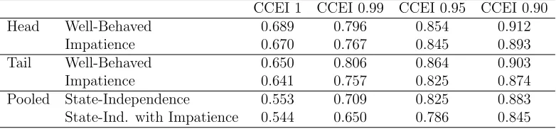
Table 2: Impatience and State-Independent Time Preference.

CCEI 1 CCEI 0.99 CCEI 0.95 CCEI 0.90 Head Well-Behaved 0.689 0.796 0.854 0.912

well-behaved utility function in state Head and similar proportion in state Tail; if impatience is imposed on the utility function, the pass rate drops (as it must) but very modestly. (Recall from Section 3.2 that the existence of well-behaved sub-utility function in state k can be ascertained by testing GARP on Osk and the existence of a well-behaved and impatient

sub-utility function in that state can be ascertained by testing a stronger version of GARP.) We also repeat the tests pooling the data in the two states, in order to test for the existence of a state independent sub-utility function; in this case, the pass rate is around 82 percent and dropping slightly to 79 percent when impatience is imposed.7

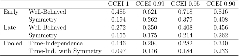
Table 3: Symmetry and Time-Invariant Risk Preference.

CCEI 1 CCEI 0.99 CCEI 0.95 CCEI 0.90 Early Well-Behaved 0.485 0.621 0.718 0.816

Symmetry 0.194 0.262 0.379 0.408 Late Well-Behaved 0.272 0.350 0.408 0.456 Symmetry 0.155 0.175 0.214 0.262 Pooled Time-Independence 0.146 0.204 0.282 0.340 Time-Ind. with Symmetry 0.097 0.146 0.184 0.233

When a subject has an overall utility function that is weakly separable across time (see (7)), he or she would have a sub-utility function at each date. This means that there are sub-utility functionsω (ωe) rationalizing the datasets Ot1 (Ot2). Table 3 reports the results of

the revealed preference tests at each time point. At the CCEI level of 0.95, 72 percent of all subjects exhibit behavior rationalizable by a well-behaved utility function at the Early time point, with the corresponding figure at the Late time point being 41 percent. These numbers drop to 38 percent and 21 percent respectively after imposing symmetry. To check for the existence of a time-invariant sub-utility function, we pool the observations (for each subject) at the two time points into a single data set; in this case, 28 percent are rationalizable with a well-behaved utility function, and the figure drops to 18 percent if symmetry is imposed.

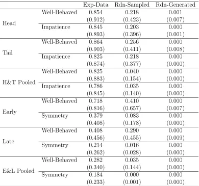
It is clear from Tables 2 and 3 that while there is strong support for the existence of sub-utility functions over consumption streams, the evidence in favor of the existence of sub-utility functions over contingent consumption (at each date) is a lot weaker. Table 4 reinforces these findings by comparing the pass rates for each test with its power. The latter is measured in two ways. In the first way, we generate datasets (each consisting of 41 observations) using random allocation decisions in which the tokens sum up to 100. In the second way, we first pool the decisions made by all subjects in the experiment and then generate datasets (of 41 observations each) by sampling from that set. Notice that for datasets randomly generated according to the first method, the pass rate is essentially zero at the

7

Table 4: Power Test.

Exp-Data Rdm-Sampled Rdm-Generated

Head Well-Behaved 0.854 0.218 0.001

Impatience 0.845 0.203 0.000

Tail Well-Behaved 0.864 0.256 0.000

Impatience 0.825 0.218 0.000

H&T Pooled Well-Behaved 0.825 0.040 0.000

Impatience 0.786 0.035 0.000

Early Well-Behaved 0.718 0.410 0.000

Symmetry 0.379 0.083 0.000

Late Well-Behaved 0.408 0.290 0.000

Symmetry 0.214 0.016 0.000

E&L Pooled Well-Behaved 0.282 0.035 0.000

Symmetry 0.184 0.000 0.000

Note. The table displays the pass rates (at CCEI 0.95) among experimental data, randomly sampled data (using subject choices) and randomly generated data. The experimental data consists of 103 datasets (from 103 subjects). For the randomly sampled data and randomly generated data, estimated pass rates are obtained from more than 10000 generated datasets in each case.

0.95 CCEI. For datasets randomly generated according to the second method, the pass rates are higher but still low when compared against the pass rate (among subjects). Selten (1991) proposes using the difference between the experimental pass rate and the pass rate from randomly generated data as a measure of a model’s predictive power.8

Notice that all the models (whether they involve state or time separability) dohave predictive power in the sense that the true pass rate exceeds the pass rates of the randomly generated data. Furthermore, the state-separable hypothesis with state independence and impatience is obviously superior in predictive power to the time-separable hypothesis with date independence and symmetry, since 0.786−0.035>0.184−0.000.

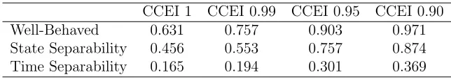
Table 5: GARP and Separability.

CCEI 1 CCEI 0.99 CCEI 0.95 CCEI 0.90 Well-Behaved 0.631 0.757 0.903 0.971 State Separability 0.456 0.553 0.757 0.874 Time Separability 0.165 0.194 0.301 0.369

So far we have only checked whether datasets are consistent with the existence of sub-utility functions, but have not actually tested whether each subject’s dataset is rationalizable by a weakly separable utility function (either of the state-separable form (6) or the time-separable

8

form (7)), which requires the recovery, not just of sub-utility functions, but also of an aggregator function. Table 5 displays the results of implementing the rationalizability test for weakly separable utility functions proposed in Quah (2014). Notice that both state-separable and time-separable utility functions are special cases of well-behaved utility functions and therefore the pass rate of the latter (which exceeds 90 percent at CCEI of 0.95) must be higher than the other two. However, while 75 percent of all subjects display behavior consistent with a state separable utility function, the corresponding figure for time separable utility is only 30 percent.

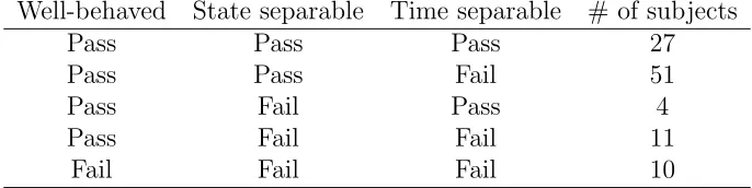
Table 6: Individual Type Analysis (pass rates at CCEI 0.95)

Well-behaved State separable Time separable # of subjects

Pass Pass Pass 27

Pass Pass Fail 51

Pass Fail Pass 4

Pass Fail Fail 11

Fail Fail Fail 10

This disparity is in some ways even more starkly displayed in Table 6, which counts the number of subjects who pass/fail the three models (at CCEI of 0.95). Notice that while 51 subjects are consistent with the state-separable model but not the time-separable model, only four subjects are consistent with the time-consistent model but not the state-separable model. So the usefulness of the model in explaining subject behavior appears to be very modest and certainly pales in comparison with the state-separable model.

5

Conclusion

We conduct an experiment to elicit preferences of subjects over risky consumption streams. Using recently developed revealed preference tests, we check for the consistency of subject behavior with a variety of preference hypotheses. Our results broadly support the hypothesis that intertemporal preferences under risk are separable across states, but there is little evidence to support separability across time. This is the source of the failure of the discounted expected utility model to explain subject behavior. Furthermore, we find that the sub-utility functions over consumption streams are state independent and exhibit impatience.

trades off between ex ante and ex post fairness concerns; ex ante fairness would suggest a preference that is separable across individuals, while ex post fairness suggests a preference that is separable across states.

REFERENCES

[1] Abdellaoui, M., H. Bleichrodt, O. l’Haridon, and C. Paraschiv (2013): “Is There One Unifying Concept of Utility? An Experimental Comparison of Utility under Risk and Utility over Time,” Management Science, 59(9): 2153-69.

[2] Afriat, S. N. (1967): “The construction of utility functions from expenditure data,”

International economic review, 8(1): 67-77.

[3] Afriat, S. N. (1972): “Efficiency estimation of production functions,” International Economic Review, 13(3): 568-598.

[4] Andreoni, J., and J. Miller (2002): “Giving according to GARP: An experimental test of the consistency of preferences for altruism,” Econometrica, 70(2): 737-753.

[5] Andreoni, J., and C. Sprenger (2012a): “Estimating Time Preferences from Convex Budgets,” American Economic Review, 102(7): 3333-56

[6] Andreoni, J., and C. Sprenger (2012b): “Risk Preferences are not Time Preferences.”

American Economic Review, 102(7): 3357-76.

[7] Augenblick, N., M. Niederle, and C. Sprenger (2015): “Working over Time: Dynamic Inconsistency in Real Effort Tasks,” The Quarterly Journal of Economics, 130(3): 1067-1115.

[8] Brock, J. M., A. Lange, and E. Y. Ozbay (2013): “Dictating the risk: Experimental evidence on giving in risky environments,” American Economic Review, 103(1): 415-437. [9] Chakraborty, A., E. M. Calford, G. Fenig, and Y. Halevy (2016): “External and

internal consistency of choices made in convex time budgets,” Experimental Economics,

forthcoming

[10] Chew, S. H., and L. G. Epstein (1990): “Non-expected Utility Preferences in a Tem-poral Framework with an Application to Consumption-Savings Behaviour,” Journal of Economic Theory, 50(1): 54-81.

[11] Choi, S., R. Fisman, D. Gale, and S. Kariv (2007): “Consistency and heterogeneity of individual behavior under uncertainty,” American Economic Review 97(5): 1921-1938. [12] Choi, S., S. Kariv, W. M¨uller, and D. Silverman (2014): “Who is (more) rational?”

American Economic Review 104(6): 1518-1550.

[13] Echenique, F., K. Saito, and T. Imai (2015): “Testable Implications of Models of Intertemporal Choice: Exponential Discounting and Its Generalizations,”working Paper

[14] Epper, T., and H. Fehr-Duda (2015) “Balancing on a Budget Line: Comment on Andreoni and Sprenger’s ‘Risk Preferences Are Not Time Preferences’,” American Economic Review, 105(7): 2261-2271.

[16] Epstein, L. G., and S. E. Zin (1991): “Substitution, risk aversion, and the temporal behavior of consumption and asset returns: An empirical analysis,” Journal of political Economy, 99(2): 263-286.

[17] Fisman, R., S. Kariv, and D. Markovits (2007): “Individual preferences for giving,”

American Economic Review,97(5): 1858-1876.

[18] Fudenberg, D., and D. K. Levine (2012): “Fairness, risk preferences and independence: Impossibility theorems,” Journal of Economic Behavior & Organization,81(2): 606-612. [19] Halevy, Y. (2014): “Some Comments on the Use of Monetary and Primary Rewards in

the Measurement of Time Preferences,” working Paper

[20] Halevy, Y. (2008): “Strotz Meets Allais: Diminishing Impatience and the Certainty Effect,” American Economic Review, 98(3): 1145-62.

[21] Kreps, D. M., and E. L. Porteus (1978): “Temporal Resolution of Uncertainty and Dynamic Choice Theory,” Econometrica, 46(1): 185-200.

[22] Nishimura, H., E. A. Ok, and J. K.-H. Quah (2017): “A comprehensive approach to revealed preference theory,” American Economic Review, 107(4): 1239-1263.

[23] Polisson, M., J. K-H. Quah, and L. Renou (2015): “Revealed preferences over risk and uncertainty,” No. W15/25. IFS Working Papers.

[24] Quah, J. K-H. (2014): “A test for weakly separable preferences,” Working Paper, Department of Economics, Oxford, No. 708.

[25] Reuben, E., P. Sapienza, and L. Zingales (2010): “Time Discounting for Primary and Monetary Rewards,” Economics Letters, 106(2): 125-27.

[26] Saito, K. (2013): “Social preferences under risk: Equality of opportunity versus equality of outcome,” American Economic Review, 103(7): 3084-3101.

[27] Selden, L. (1978): “A New Representation of Preferences over Certain X Uncertain Consumption Pairs: The Ordinal Certainty Equivalent Hypothesis,”Econometrica, 46(5): 1045-60.

[28] Selten, R. (1991): “Properties of a Measure of Predictive Success,” Mathematical Social Sciences, 21(2): 153-167.

[29] Varian, H. R. (1982): “The nonparametric approach to demand analysis,” Econometrica, 50(4): 945-973.

Appendix: Supplementary Tables

Table A1: Price Effect with only Interior Choices.

Head/Early Tail/Early Head/Late Tail/Late allocation allocation allocation allocation Head/Early Price -9.247*** 3.149*** 5.900*** 0.198

(1.802) (1.014) (1.214) (0.924) Tail/Early Price -0.105 -8.904*** 3.084*** 5.925***

(0.937) (1.552) (0.776) (1.259) Head/Late Price 5.730*** 1.683* 9.986*** 2.572***

(1.259) (0.993) (1.693) (0.830) Tail/Late Price 1.440* 7.251*** 1.144 -9.836***

(0.762) (1.550) (0.706) (1.598) constant 27.803*** 21.167*** 24.621** 26.409***

(2.015) (2.353) (1.997) (2.218)

Observations 984 984 984 984

Pseudo R-squared 0.210 0.248 0.236 0.242

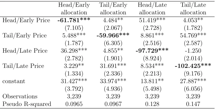
Table A2: Price Effect with only Corner Choices.

Head/Early Tail/Early Head/Late Tail/Late allocation allocation allocation allocation Head/Early Price -61.781*** 4.484** 51.419*** 4.053**

(7.105) (2.067) (2.728) (1.782) Tail/Early Price 5.488*** -59.966*** 8.861*** 54.769***

(1.787) (6.305) (2.516) (2.587) Head/Late Price 36.298*** 4.855** -97.729*** -1.250 (2.782) (1.901) (8.924) (2.014) Tail/Late Price 3.229** 31.691*** 8.534*** -102.425***

(1.334) (2.336) (2.213) (9.176) constant 31.427*** 33.974*** 13.811** 27.887***

Table A3: Power Test (at CCEI 0.95 and 0.90)

Exp-Data Rdn-Sampled Rdn-Generated

Head

Well-Behaved 0.854 0.218 0.001

(0.912) (0.423) (0.007)

Impatience 0.845 0.203 0.000

(0.893) (0.396) (0.001)

Tail

Well-Behaved 0.864 0.256 0.000

(0.903) (0.411) (0.008)

Impatience 0.825 0.218 0.000

(0.874) (0.377) (0.000)

H&T Pooled

Well-Behaved 0.825 0.040 0.000

(0.883) (0.154) (0.000)

Impatience 0.786 0.035 0.000

(0.845) (0.140) (0.000)

Early

Well-Behaved 0.718 0.410 0.000

(0.816) (0.657) (0.007)

Symmetry 0.379 0.083 0.000

(0.408) (0.178) (0.000)

Late

Well-Behaved 0.408 0.290 0.000

(0.456) (0.455) (0.009)

Symmetry 0.214 0.016 0.000

(0.262) (0.028) (0.000)

E&L Pooled

Well-Behaved 0.282 0.035 0.000

(0.340) (0.144) (0.000)

Symmetry 0.184 0.000 0.000

(0.233) (0.001) (0.000)

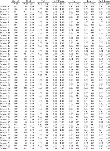
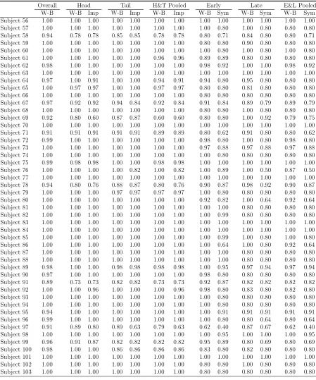
Table A4: Detailed CCEI Results.

Overall Head Tail H&T Pooled Early Late E&L Pooled

W-B W-B Imp W-B Imp W-B Imp W-B Sym W-B Sym W-B Sym

Table A4 continued.

Overall Head Tail H&T Pooled Early Late E&L Pooled

W-B W-B Imp W-B Imp W-B Imp W-B Sym W-B Sym W-B Sym