Munich Personal RePEc Archive
Forecasting Financial Vulnerability in the
US: A Factor Model Approach
Kim, Hyeongwoo and Shi, Wen
Auburn University, Columbus State University
October 2018
Forecasting Financial Vulnerability in the US:
A Factor Model Approach
Hyeongwoo Kim
∗Auburn University
Wen Shi
†Columbus State University
October 2018
Abstract
This paper presents a factor-based forecasting model for the financial mar-ket vulnerability, measured by changes in the Cleveland Financial Stress Index (CFSI). We estimate latent common factors via the method of the principal components from 170 monthly frequency macroeconomic data in order to out-of-sample forecast the CFSI. Our factor models outperform both the random walk and the autoregressive benchmark models in out-of-sample predictability at least for the short-term forecast horizons, which is a desirable feature since financial crises often come to a surprise realization. Interestingly, the first com-mon factor, which plays a key role in predicting the financial vulnerability index, seems to be more closely related with real activity variables rather than nominal variables. We also present a binary choice version factor model that estimates the probability of the high stress regime successfully.
Keywords: Financial Stress Index; Method of the Principal Component;
Out-of-Sample Forecast; Ratio of Root Mean Square Prediction Error;
Diebold-Mariano-West Statistic; Ordered Probit Model
JEL Classification: E44; E47; G01; G17
∗Patrick E. Molony Professor of Economics, Department of Economics, Auburn University,
138 Miller Hall, Auburn, AL 36849. Tel: +1-334-844-2928. Fax: +1-334-844-4615. Email: [email protected].
†Contact Author: Wen Shi, Department of Accounting & Finance, Turner College of Business,
1
Introduction
Financial market crises often occur abruptly, then quickly spread to other sectors of the economy. As Reinhart and Rogo¤ (2014) point out, harmful e¤ects of …nancial crises on the real sectors of the economy tend to be severe because recessions that result from …nancial market crises are likely to persist for a long period of time.
The recent global recession that ensued from the collapse of the US …nancial market in 2008 provides a stark reminder of the danger of …nancial crises. Unfortunately, the profession has failed to anticipate it, and greatly underestimated the severity of the spillover e¤ect of the crisis to real activity that resulted in the Great Recession. For this reason, it would be useful to have an early-warning system (EWS) that alerts …nancial market participants to incoming danger before it occurs (Reinhart and Rogo¤ (2009)).
Designing EWS’ naturally requires an appropriate measure of the …nancial vul-nerability which quanti…es the potential risk that may become prevalent in …nancial markets. One may consider using the Exchange Market Pressure (EMP) index that has been frequently employed by researchers since the seminal work of Girton and Roper (1977).1 The EMP index, however, may not be ideal to study the …nancial distress in
a large economy such as the US, because it is based on changes in exchange rates and reserves. That is, it may be more suitable for small open economies.
One alternative measure that is rapidly gaining popularity is a …nancial stress index (FSI). Unlike the EMP index, FSI’s are constructed using a broad range of key …nancial market variables. In the US, 12 …nancial stress indices have currently become available (Oet, Eiben, Bianco, Gramlich, and Ong (2011)) since the recent …nancial crisis, including the three FSI’s contributed by regional Federal Reserve banks. See, among others, Hakkio and Keeton (2009), Kliesen and Smith (2010), Oet, Eiben, Bianco, Gramlich, and Ong (2011), and Brave and Butters (2012).
Conventional approaches to predict …nancial crises include the following. Frankel and Saravelos (2012), Eichengreen, Rose, and Wyplosz (1995), and Sachs, Tornell, and Velasco (1996) use linear regression approaches to test the statistical signi…cance of various economic variables on the occurrence of crises. Others employ discrete choice models including parametric probit or logit models (Frankel and Rose (1996); Cipollini and Kapetanios (2009)) and nonparametric signals approach (Kaminsky, Lizondo, and Reinhart (1998); Brüggemann and Linne (1999); Edison (2003); Berg and Pattillo
(1999); Bussiere and Mulder (1999); Berg, Borensztein, and Pattillo (2005); EI-Shagi, Knedlik, and von Schweinitz (2013); Christensen and Li (2014)).
This paper presents factor-based out-of-sample forecasting approach for the Cleve-land Financial Stress Index (CFSI) developed by the CleveCleve-land Fed. We estimate multiple latent common factors via the method of the principal components (Stock and Watson (2002)) to a large panel of 170 time series macroeconomic data that in-clude nominal and real activity variables from October 1991 to October 2014. To avoid potential issues that are associated with nonstationarity of the data, we apply the principle component analysis (PCA) to …rst-di¤erenced data, then recover level
factors from estimateddi¤erenced factors (Bai and Ng (2004)). Then, we augment an autoregressive (AR) type model with estimated common factors.
To evaluate the out-of-sample prediction performance of our models, we implement an array of forecast exercises with the random walk (RW) as well as a stationary AR-type model as the benchmark. We test the equal predictability of our models relative to these benchmark models using the ratio of the root mean squared prediction errors (RRM SP E) and the Diebold-Mariano-West (DM W) test statistics.
Our major …ndings are as follows. First, our models outperform the RW benchmark model in out-of-sample forecasting for up to 1-year forecast horizons. Our models also perform better than the AR model for short-term (1 to6 month) forecast horizons. It should be noted that this is a desirable feature since …nancial crises often occur abruptly with no prior warnings. Second, parsimonious models with just one or two factors perform as well as bigger models that use up to 8 factors. Third, the …rst common factor that plays a key role in our forecast exercises seems to be closely related with real sector variables rather than nominal variables. That is, real activity variables provide useful predictive contents for the …nancial vulnerability.
2
The Econometric Model
Letxi;t be a macroeconomic time series variable that is characterized by the following
factor structure. Abstracting from deterministic terms, we assume the following factor structure:
xi;t =
0
iFt+ei;t; i= 1;2; ::; N; t= 1;2; ::; T; (1)
whereFt= [F1;t Fr;t]
0
is not directly observable (latent)common factors and i =
[ i;1 i;r]
0
denotes ith variable speci…c, time invariant factor loading coe¢cients.
Note that 0iFt jointly determines the dependency ofxi;t on the common factors, while
ei;t is the idiosyncratic error term. All variables except those that are represented as
percentage (e.g., interest rates and unemployment rates) are log-transformed.
Estimation is carried out via the method of the principal components for the …rst-di¤erenced data. As Bai and Ng (2004) show, the principal component estimators for
Ft and i are consistent irrespective of the order of Ft as long as ei;t is stationary.
However, ifei;t is an integrated process, a regression ofxi;t onFt is spurious. To avoid
this problem, we apply the method of the principal components to the …rst-di¤erenced data. That is, we rewrite (1) by the following.
xi;t =
0
i Ft+ ei;t (2)
for t = 2; ; T. Let xi = [ xi;1 xi;T]
0
and x = [ x1 xN]. We …rst
normalize the data prior to estimations, since the method of the principal components is not scale invariant. Taking the principal components method for x x0 yields factor estimates F^t along with their associated factor loading coe¢cients ^i. Estimates for
the idiosyncratic components are naturally given by the residuals e^i;t = xi;t ^
0
i F^t.
Level variables are recovered by re-integrating these estimates. That is,
^
ei;t = t
X
s=2 ^
ei;s (3)
fori= 1;2; :::; N. Similarly,
^
Ft =
t
X
s=2
^
Fs (4)
the following model,
f sit+j =
0
^
Ft+ jf sit+ut+j; j = 1;2; ::; k; (5)
where j is the coe¢cient on thecurrent FSI for thej-period ahead FSI. That is, we
im-plementdirect forecasting scheme for f sit+j on (di¤erenced) common factor estimates
( F^t) and f sit, which are assumed to belong to the econometrician’s information set
( t) at time t. Note that (5) is an AR(1) process for j = 1, augmented by
exoge-nous common factor estimates. This formulation is based on our preliminary unit-root test results for the FSI that show strong evidence of stationarity.2 Applying the least
squares (LS) estimation for (5), we obtain the following j-period ahead forecast from our factor (F) model.
c
f siFt+jjt = ^
0 ^
Ft+ ^jf sit; (6)
where ^and ^j are the LS estimates.
To statistically evaluate the out-of-sample predictability performance of our factor models, we employ the following nonstationary random walk (RW) model that serves the (no change) benchmark model.
f sit+1 =f sit+"t+1 (7)
It is straightforward to see that (7) yields the following j-period ahead forecast.
c
f siRWt+jjt =f sit; (8)
wheref sit is the current value of the …nancial stress index.
In addition, we employ the following stationary AR(1)-type forecasting model as an alternative benchmark model.
f sit+j = jf sit+"t+1; (9)
which yields the following j-period ahead forecast.
c
f siARt+jjt = ^jf sit; (10)
For evaluation criteria, we use the ratio of the root mean squared prediction error (RRM SP E), which is de…ned as the root mean squared prediction error (RM SP E) from the benchmark model divided byRM SP E from our factor model. Note that our factor model outperforms the benchmark model whenRRM SP E is greater than 1.
We also employ the Diebold-Mariano-West (DM W) test. For this, we de…ne the following loss di¤erential function.
dt=L("At+jjt) L(" F
t+jjt); (11)
whereL( ) is a loss function based on forecast errors under each model. That is,
"Bt+jjt=f sit+j f sic B
t+jjt (B =RW; AR); " F
t+jjt=f sit+j f sic F
t+jjt (12)
One may use either the squared error loss function,("jt+jjt)
2
, or the absolute loss func-tion, j"jt+jjtj.
The following DM W statistic can be used to test the null hypothesis of equal predictive accuracy, H0 :Edt = 0,
DM W = q d
[
Avar(d)
; (13)
wheredis the sample mean loss di¤erential function,d= 1
T T0
PT
t=T0+1dt, andAvar[(d) denotes the asymptotic variance ofd,
[
Avar(d) = 1
T T0
q
X
i= q
k(i; q)^i (14)
k( ) is a kernel function where T0=T is the split point in percent, k( ) = 0; j > q, and ^j is jth autocovariance function estimate.3
Note that our factor model (5) nests the stationary benchmark model in (9). There-fore, we use critical values proposed by McCracken (2007) for this case. For theDM W
statistic with the random walk benchmark (7), which is not nested by (5), we use the asymptotic critical values, which are obtained from the standard normal distribution.
3T
0 is the number of initial observations that are used to formulate the …rst out-of-sample
3
Data Descriptions and Factor Estimations
3.1
Data Descriptions
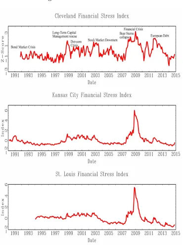
We use the Cleveland Financial Stress Index (CFSI) to measure the …nancial market vulnerability. We obtained the data from the FRED. Observations are monthly and are available from October 1991. The CFSI is designed to track …nancial distress in the US on a continuous basis. The index integrates 11 daily …nancial market indicators which are grouped into four sectors: debt, equity, foreign exchange, and banking. See Oet, Eiben, Bianco, Gramlich, and Ong (2011) for details. Units of the CFSI are expressed asz-scores and a high value of the CFSI indicates an elevated level of systemic …nancial stress. For example, a score higher than 0.544 implies a moderate to signi…cant stress period.
As we can see in Figure 1, the CFSI traces past episodes of …nancial distress in the US quite well. For instance, the CFSI increases rapidly during the turbulent periods such as the Long-Term Capital Management (LTCM) crisis in the late 1990’s. The CFSI began picking up an elevated …nancial distress since late 2007. The index reached 2.42 when the Bear Stearns collapsed and sold to JPMorgan in March 2008, then peaked in December 2008 after the failure of Lehman Brothers in September of the same year. We observe a similarly sharp rise of the index during the European debt crisis in the early 2010’s. Overall, the CFSI seems to be an appropriate measure of the …nancial vulnerability.
Figure 1 around here
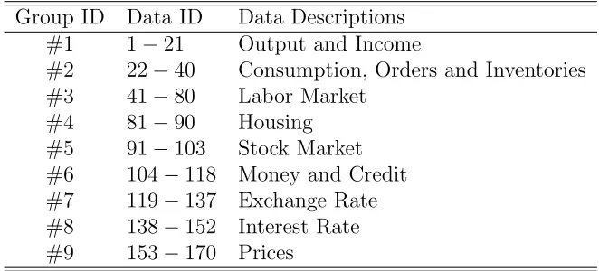
We obtained 170 monthly frequency macroeconomic time series data from the FRED and the Conference Boards Indicators Database. Observations span from Oc-tober 1991 to OcOc-tober 2014 to match the availability of the CFSI. We organized these 170 time series data into 9 small groups as summarized in Table 1. Groups #1 through #5 (Data ID #1 to #103) are variables that are closely related with real sector ac-tivity, while groups #6 to #9 (Data ID #104 to #170) are mostly nominal variables. Detailed explanations on individual time series are reported in the appendix.
3.2
Latent Factors and their Characteristics
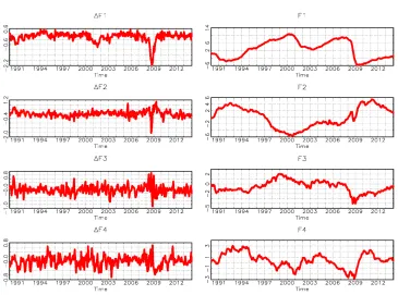
We estimated up to 8 latent common factors via the method of the principal compo-nents for the …rst-di¤erenced data. In Figure 2, we report …rst four (di¤erenced) com-mon factor estimates, F1; F2; F3; F4 and their level counterparts F1; F2; F3; F4,
obtained by re-integrating these di¤erenced factors. One notable observation is that the …rst common factor F1 exhibits rapid declines around 2001 and 2008, which
cor-respond to a recession after the burst of the US IT bubble (so-called, the dot-com bubble) and the recent Great Recession, respectively. In what follows, we demonstrate that F1 is more closely related with real sector variables, though it also represent a
group of nominal variables as well.
Figure 2 around here
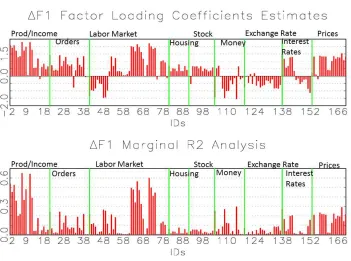
We report the factor loading coe¢cient ( i) estimates and marginal R2 of each
variable in Figures 3 to 6 to study how each of these factors is associated with the macroeconomic variables in groups #1 to #9. The marginal R2
is an in-sample …t statistic obtained by regressing each of the individual time series variables onto each estimated common factor, one at a time, using the full sample data. The individual series in each group are separated by vertical lines and labeled by group ID’s. The individual data ID’s are on the x-axis and the descriptions are reported in the Data Appendix.
We …rst investigate the nature of the …rst common factor using the factor loading coe¢cients for F1. It should be noted that loading coe¢cients of most variables in
As to the marginal R2
estimation, F1 explains a substantial portion of variations
in measures of production and the employment part in the labor market, even though it also explain non-negligible portions of variations in price variables as well. Overall,
F1 seems to better represent real activity performance.
Figure 3 around here
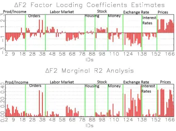
As we can see in Figure 4, the second common factor F2 seems to be highly
cor-related with the group #9 (price variables) as well as the group #7 (exchange rates). That is, the marginal R2
values of these variables are far greater than those of other variables. Factor loading coe¢cients of these variables are similar to those in Figure 3 and tend to be bigger in absolute terms than other coe¢cients. Therefore,F2 seems to
be more closely associated with the two groups of nominal variables, domestic prices and foreign exchange rates.
Figure 4 around here
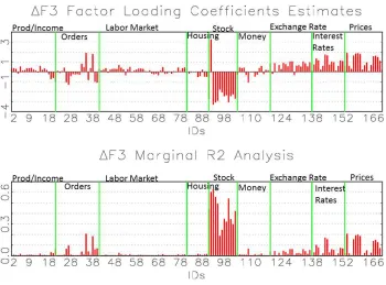
F3 seems to re‡ect mainly the information on the group #5 stock price variables.
As we can see in the marginal R2
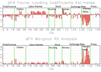
analysis, it explains over 60% of variations in these variables. The loading coe¢cient estimates are mostly negative except the …rst one in this group, the price-earning ratio (earnings/price), which makes sense because the stock price appears in the denominator. Similar reasoning implies that the group #8 variables (interest rates) are well explained byF4.
Figures 5 and 6 around here
4
Forecasting Exercises
4.1
In-Sample Fit Analysis
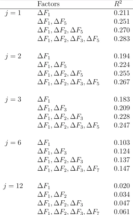
We employ an R2
-based selection method considering one-factor model to the 8-factor full model to …nd good combinations of explanatory variables. The …rst common factor F1 seems to play the most important role in explaining variations in the CFSI
for all forecasting time horizons we consider.
We note that adding more factors after the …rst common factor does not sub-stantially increase the goodness of …t. That is, one or two factor models seem to be su¢cient for a good in-sample …t. It should be also noted that factor estimates help explain CFSI’s in relatively short time horizons. For example, factors explain 20 to
30%variations in1 month ahead CFSIs, while they explain less than10%of variations in1 year ahead CFSIs even with full 8 factor models.4
Table 2 around here
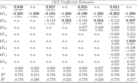
In Table 3, we report the LS estimates of the coe¢cients in the regression model of the1 period ahead CFSI index (cf sit+1). We note that the …rst common factor is
highly signi…cant whether one period lagged CFSI (cf sit) is included in the regression
or not. The second common factor also plays an important role when pure factor models withoutcf sit are employed. Our models provides good in-sample …t especially
when cf sit is included, although our models still exhibit fairly good in-sample …t
performance without it.5 The 8 factor full model explains roughly 30% of variation
of the one-month ahead CFSI.
Table 3 around here
4.2
Out-of-Sample Forecast Exercises and Evaluations of the
Models
We evaluate the out-of-sample predictability of our factor models using the following two methods. First, we employ a recursive forecast scheme. That is, we begin with
4We also considered alternative factor selection methods. For instance, the adjusted R2
selection method usually chose the5 or6 factor model, while a stepwise selection method (Speci…c-to-General
rule) selected the4 or5 factor model for the FSI. However, added gains are still fairly small.
an out-of-sample forecast of thej period ahead CFSI index (f siT0+j) using the initial 50% observations (t= 1;2; :::; T0; T0 = T2). Then, we add one next observation to the
sample (t= 1;2; :::; T0; T0 + 1), and implement another forecast (f siT0+j+1) using new estimates from this expanded set of observations. We repeat this until we forecast the last observations. We implement this scheme for up to 12 month forecast horizons,
j = 1;2;3;6;12.
The second scheme is a …xed-size rolling window method that repeats forecasting by adding one next observation with the same split point (50% or T0 = T2), but dropping
one earliest observation in order to maintain the same size of the window. That is, after the initial forecast described earlier, we forecastf siT0+j+1 using an updated (shifted to the right) data set (t = 2;3; :::; T0; T0+1) maintaining the same number of observations.
As we described in the previous section, we employ the following two benchmark models: the nonstationary random walk (RW) model and a stationary autoregressive (AR) model. Out-of-sample forecast performance is evaluated using the ratio of the root mean square prediction error,RRM SP E. Also, we implement the DM W test to statistically evaluate prediction accuracy of our models.
RRM SP E estimates of our factor models relative to the random walk benchmark are reported in Table 4. We note that our factor models outperform the benchmark model for all forecast horizons from 1 month to 1 year. TheRRM SP E estimates are greater than one for all cases both with the recursive and the rolling window schemes. Similarly as in the in-sample …t analyses reported earlier, one factor model with the …rst common factor F1 performs as well as bigger models with more factor estimates.
The DM W statistics are reported in Table 5. Using the asymptotic critical values from the standard normal distribution, the test rejects the null hypothesis of equal predictive accuracy at the 10% signi…cance level in majority cases when the forecast horizon is 3 month or longer. For shorter forecast time horizon (1 and 2 month), the test rejects the null for just one case even though the test statistic is all positive meaning that the test favors the factor models.
Tables 4 and 5 around here
1 and 6 month. The RRM SP E was all less than one for 12 month ahead out-of-sample forecast. It should be noted, however, that short-term forecast accuracy is more desirable feature for predicting the …nancial market vulnerability, because …nancial crises often occur abruptly.
Note that our factor models nest the benchmark AR model, which results in size distortion when the asymptotic critical values are used. Based on the critical values from McCracken (2007), the DM W test rejects the null hypothesis for most cases at the 10% signi…cance level when the forecast horizon is shorter than 12 month, which is consistent with the results in Table 6.
Tables 6 and 7 around here
5
An Ordered Probit Model Approach
This section presents an ordered probit model version factor model by transforming
f sit into a binary variable that takes either 1 (high …nancial stress: H) or 0 (low
…nancial stress: L) values. Following the guideline from the Cleveland Fed, we assume that the US …nancial market is under the high …nancial stress regime when f sit is
greater than0:544, while it is under the low …nancial stress regime otherwise.6
For such a two-regime probit model, we consider the following latent equation:
yt =x
0
t "t; (15)
where yt is unobservable latent variable with an r 1 vector of covariates xt =
[ F1;t; :::; Fr;t]
0
. "t is assumed to obey the standard normal distribution.
Let yt denote the observable state variable from this latent equation. When yt is
greater than the threshold , we observe the high stress regimeH (yt = 1). Otherwise,
the low stress regimeL is realized, yt = 0. That is,
yt=
( 1;
0;
if if
yt > yt <
:H
:L (16)
6The Cleveland Fed provides three threshold values for 4 regimes: low stress, normal stress,
The log-likelihood function for a random sample of sizeT, fytgTt=1, is the following. L= T X t=1 h
I(yt= 1) ln F x
0
t +I(yt= 0) ln 1 F x
0
t
i
; (17)
whereI( )is the indicator function and F( )is the standard normal distribution func-tion.
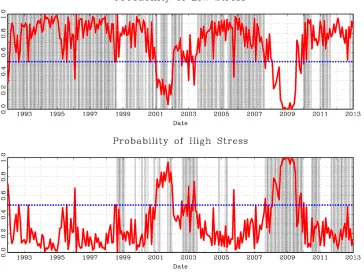
We estimated (17) via the method of the maximum likelihood estimation using the two factor estimates F1 and F2.7 We report the probability estimates of the two
regimes,H and L, in Figure 7. Bar graphs indicate actual realizations of the regimes from the data using the threshold 0:544. Our factor model seems to perform well in this framework too, because estimated probabilities trace changes in the state of the …nancial vulnerability fairly well over time. For example, the estimated probability of the regime H rapidly increases during the recent …nancial crisis, whereas the low regime probability stays high in the 1990’s.
Figure 7 around here
6
Concluding Remarks
This paper proposes a factor-based forecasting model for systemic risk in the U.S. …-nancial market in a data-rich environment. We use the ……-nancial stress index developed by Federal Reserve Bank of Cleveland to measure the …nancial vulnerability. We em-ploy a dimensionality reduction method that extracts multiple latent common factors from a panel of 170 monthly frequency time series macroeconomic variables from Oc-tober 1991 to OcOc-tober 2014. In the presence of nonstationarity in the data, we apply the method of the principle components (Stock and Watson (2002)) to …rst-di¤erenced data (Bai and Ng (2004)) to estimate the latent factors consistently. Our factor models augment an AR-type self-exciting process of the Cleveland Financial Stress Index with estimated common factors.
To evaluate the practical usefulness of our factor models, we implement an array of out-of-sample prediction exercises using the recursive and the …xed-size rolling window schemes for 1-month to 1-year forecast horizons. Based on the RRM SP E estimates
7Models with one or three factor estimates yield qualitatively similar results. All results are
and the DM W statistics, our factor-based forecasting models overall outperform the nonstationary random walk benchmark model as well as the stationary autoregressive model especially for short-horizon predictions, which is a desirable feature because …nancial crises often come to a surprise realization. Parsimonious models with just one or two factors performed as well as bigger models in providing potentially useful information to policy makers and …nancial market participants. Interestingly, real activity variables represented by the …rst common factor are shown to have substantial predictive contents for the …nancial market vulnerability even in the short-run.
References
Andrews, D. W. K.,andJ. C. Monahan(1992): “An Improved Heteroskedasticity
and Autocorrelation Consistent Covariance Matrix Estimator,”Econometrica, 60(4), 953–966.
Bai, J., and S. Ng (2004): “A PANIC Attack on Unit Roots and Cointegration,”
Econometrica, 72, 1127–1177.
Berg, A., E. Borensztein, and C. Pattillo (2005): “Assessing Early Warning Systems: How Have They Worked in Practice?,” IMF Working Paper 04/52. Inter-national Monetary Fund.
Berg, A., and C. Pattillo (1999): “Predicting Currency Crises: The Indicators
Approach and an Alternative,”Journal of International Money and Finance, 18(4), 561–586.
Brave, S.,and R. A. Butters(2012): “Diagnosing the Financial System: Financial Conditions and Financial Stress,” The international Journal of Central Banking, 8(2), 191–239.
Brüggemann, A., and T. Linne (1999): “How Good are Leading Indicators for Currency and Banking Crises in Central and Eastern Europe? An Empirical Test,” IWH Discussion Papers, 95.Halle Institute for Economic Research.
Bussiere, M.,and C. Mulder(1999): “External Vulnerability in Emerging Market Economies - How High Liquidity Can O¤set Weak Fundamentals and the E¤ects of Contagion,” IMF Working Papers 99/88.
Christensen, I., and F. Li (2014): “Predicting Financial Stress Events: A Signal Extraction Approach,” Working Paper 2014-37. Bank of Canada.
Cipollini, A.,and G. Kapetanios (2009): “Forecasting Financial Crises and
Con-tagion in Asia using Dynamic Factor Analysis,”Journal of Empirical Finance, 16(2), 188–200.
EI-Shagi, M., T. Knedlik, and G. von Schweinitz (2013): “Predicting Finan-cial Crises: The(statistical) signi…cance of the signals approach,” Journal of Inter-national Money and Finance, 35, 75–103.
Eichengreen, B., A. K. Rose, and C. Wyplosz (1995): “Exchange Market May-hem: The Antecedents and Aftermath of Speculative Attacks,”Economic Policy, 10 (21), 249–312.
Frankel, J., and G. Saravelos (2012): “Can leading indicators assess country vulnerability? Evidence from the 2008–09 global …nancial crisis,” Journal of Inter-national Economics, 87, 216 –231.
Frankel, J. A., and A. K. Rose (1996): “Currency crashes in emerging markets: an empirical treatment,” Journal of International Economics, 41 (3/4), 351–366.
Girton, and Roper (1977): “A Monetary Model of Exchange Market Pressure Ap-plied to the Postwar Canadian Experience,” American Economic Review, 67, 537– 548.
Hakkio, C. S.,andW. R. Keeton(2009): “Financial Stress:What Is It How Can It Be Measured, and Why Does It Matter?,” Economic Review, Second Quarter, 5–50.
Kaminsky, G., S. Lizondo, and C. Reinhart (1998): “Leading indicators of cur-rency crises,” IMF Working Paper No. 45 International Monetary Fund.
Kliesen, K. L., and D. C. Smith (2010): “Measuring Financial Market Stress,”
Federal Reserve Bank of St. Louis. Economic Synopses.
McCracken, M. W.(2007): “Asymptotics for out of sample tests of Granger
causal-ity,” Journal of Econometrics, 140, 719–752.
Oet, M. V., R. Eiben, T. Bianco, D. Gramlich, and S. J. Ong (2011): “The Financial Stress Index: Identi…cation of System Risk Conditions,” Working Paper No. 1130, Federal Reserve Bank of Cleveland.
Reinhart, C. M., and K. S. Rogoff (2009): This Time Is Di¤erent: Eight Cen-turies of Financial Folly, vol. 1 of Economics Books. Princeton University Press.
Sachs, J., A. Tornell, and A. Velasco (1996): “Financial Crises in Emerging Markets: The Lessons from 1995,” Brookings Papers on Economic Activity, 27(1), 147–199.
Stock, J. H., and M. W. Watson (2002): “Macroeconomic Forecasting using
Dif-fusion Indexes,” Journal of Business and Economic Statistics, 20(2), 147–162.
Figure 1. Financial Stress Indices
Note: The Cleveland Financial Stress Index is obtained from the FRED. The index is a z-score monthly frequency data constructed by the Cleveland Fed.
Figure 2. Factor Estimates: Differenced and Level Factors
Figure 3. Common Factor #1
Note: Factor loading coefficients (λi) for each common factor estimate are
Figure 4. Common Factor #2
Note: Factor loading coefficients (λi) for each common factor estimate are
Figure 5. Common Factor #3
Note: Factor loading coefficients (λi) for each common factor estimate are
Figure 6. Common Factor #4
Note: Factor loading coefficients (λi) for each common factor estimate are
Figure 7. Probability Estimation Results
Table 1. Macroeconomic Data Descriptions
Group ID Data ID Data Descriptions
#1 1−21 Output and Income
#2 22−40 Consumption, Orders and Inventories
#3 41−80 Labor Market
#4 81−90 Housing
#5 91−103 Stock Market
#6 104−118 Money and Credit #7 119−137 Exchange Rate #8 138−152 Interest Rate #9 153−170 Prices
Table 2. j-Period Ahead In-Sample R2 Fit Analysis
Factors R2
j = 1 ∆F1 0.211
∆F1,∆F5 0.251
∆F1,∆F2,∆F5 0.270 ∆F1,∆F2,∆F3,∆F5 0.283
j = 2 ∆F1 0.194
∆F1,∆F5 0.224
∆F1,∆F2,∆F5 0.255
∆F1,∆F2,∆F3,∆F5 0.267
j = 3 ∆F1 0.183
∆F1,∆F3 0.209
∆F1,∆F2,∆F3 0.228
∆F1,∆F2,∆F3,∆F5 0.247
j = 6 ∆F1 0.103
∆F1,∆F3 0.124
∆F1,∆F2,∆F3 0.137 ∆F1,∆F2,∆F3,∆F7 0.147
j = 12 ∆F1 0.020
∆F1,∆F2 0.034
∆F1,∆F2,∆F3 0.047
∆F1,∆F2,∆F3,∆F7 0.061
Table 3. OLS Estimations for the 1-Period Ahead Index (cf sit+1)
OLS Coefficient Estimates
cf sit 0.848
(26.599) n.a. 0(26.857.161) n.a. (250.855.973) n.a. 0(24.851.523) n.a.
∆F1,t −0.205
(−2.301) −1
.288 (−8.605) −0
.194 (−2.166) −1
.288 (−8.703) −0
.196 (−2.189) −1
.288 (−8.727) −0
.202 (−2.222) −1
.288 (−9.014)
∆F2,t n.a. n.a. −0.118
(−1.143) 0
.503
(2.677) −(−01..116126) 0
.504
(2.689) −(−01..112079) 0
.507 (2.793)
∆F3,t n.a. n.a. n.a. n.a. 0.077
(0.653) 0(1..349589) (00..080674) 0(1..352655)
∆F4,t n.a. n.a. n.a. n.a. n.a. n.a. −0.003
(−0.022) 0
.274
(1.262)
∆F5,t n.a. n.a. n.a. n.a. n.a. n.a. 0.042
(0.296) 1(4.050.282)
∆F6,t n.a. n.a. n.a. n.a. n.a. n.a. 0.104
(0.694) −(−00..108399)
∆F7,t n.a. n.a. n.a. n.a. n.a. n.a. −0.289
(−1.843) −0
.452
(−1.602)
∆F8,t n.a. n.a. n.a. n.a. n.a. n.a. 0.055
(0.328) 0(0..187616)
c 0.003
(0.109) 0(0..028532) 0(0..003104) 0(0..028528) 0(0..003104) 0(0..027525) (00..003096) 0(0..027526)
R2 0.782 0.213 0.783 0.234 0.783 0.241 0.786 0.301
˜
R2 0.779 0.208 0.779 0.225 0.779 0.229 0.778 0.277
Table 4. j-Period Ahead Out-of-Sample Forecast: ARF vs. RW
RRMSPE: Recursive Method
Factors/j 1 2 3 6 12
∆F1 1.021 1.040 1.057 1.099 1.120
∆F1,∆F2 1.019 1.030 1.039 1.082 1.098 ∆F1,∆F3 1.018 1.059 1.064 1.112 1.126
∆F1,∆F4 1.018 1.039 1.060 1.091 1.113
∆F1,∆F2,∆F3 1.015 1.048 1.045 1.094 1.108
RRMSPE: Rolling Window Method
Factors/j 1 2 3 6 12
∆F1 1.025 1.044 1.060 1.102 1.129
∆F1,∆F2 1.023 1.032 1.036 1.085 1.113
∆F1,∆F3 1.033 1.072 1.068 1.110 1.126 ∆F1,∆F4 1.012 1.042 1.067 1.092 1.126
∆F1,∆F2,∆F3 1.029 1.059 1.043 1.091 1.114
Note: RRMSPE denotes the mean square error from the random walk (RW)
model relative to the mean square error from our factor model (ARF). Therefore,
when RRMSPE is greater than one, our factor models perform better than the
Table 5. j-Period Ahead Out-of-Sample Forecast: ARF vs. RW
DMW: Recursive Method
Factors/j 1 2 3 6 12
∆F1 0.735 1.262 1.847∗ 2.892‡ 3.502‡
∆F1,∆F2 0.667 0.974 1.235 2.397† 2.651‡
∆F1,∆F3 0.639 1.572 1.844∗ 3.006‡ 3.268‡
∆F1,∆F4 0.661 1.228 1.899∗ 2.693‡ 3.412‡
∆F1,∆F2,∆F3 0.552 1.291 1.293 2.527† 2.679‡
DMW: Rolling Window Method
Factors/j 1 2 3 6 12
∆F1 0.833 1.271 1.835∗ 2.519‡ 2.905‡
∆F1,∆F2 0.783 0.978 1.078 2.176† 2.545†
∆F1,∆F3 1.110 1.721∗ 1.829∗ 2.501† 2.753‡
∆F1,∆F4 0.429 1.181 1.995† 2.259† 2.791‡
∆F1,∆F2,∆F3 0.988 1.485 1.148 2.100† 2.467†
Note: DMW denotes the Diebold-Mariano-West statistic. ‡, †, and ∗ indicate
Table 6. j-Period Ahead Out-of-Sample Forecast: ARF vs. AR
RRMSPE: Recursive Method
Factors/j 1 2 3 6 12
∆F1 1.013 1.013 1.019 1.008 0.973
∆F1,∆F2 1.011 1.004 1.001 0.992 0.953 ∆F1,∆F3 1.010 1.032 1.025 1.020 0.978
∆F1,∆F4 1.010 1.013 1.021 1.001 0.967
∆F1,∆F2,∆F3 1.008 1.021 1.006 1.003 0.962
RRMSPE: Rolling Window Method
Factors/j 1 2 3 6 12
∆F1 1.016 1.018 1.023 1.023 0.996
∆F1,∆F2 1.014 1.006 1.000 1.007 0.981
∆F1,∆F3 1.024 1.045 1.030 1.030 0.993 ∆F1,∆F4 1.004 1.016 1.030 1.013 0.993
∆F1,∆F2,∆F3 1.020 1.033 1.006 1.012 0.983
Note: RRMSPE denotes the mean square error from the autoregressive (AR)
model relative to the mean square error from our factor model (ARF). Therefore,
when RRMSPE is greater than one, our factor models perform better than the
Table 7. j-Period Ahead Out-of-Sample Forecast: ARF vs. AR
DMW: Recursive Method
Factors/j 1 2 3 6 12
∆F1 0.550∗ 0.531∗ 1.067† 0.594∗ -1.947
∆F1,∆F2 0.484∗ 0.181 0.060 -0.581 -2.586
∆F1,∆F3 0.436∗ 1.079† 1.219† 1.215† -1.672
∆F1,∆F4 0.450∗ 0.512∗ 1.363‡ 0.053 -2.246
∆F1,∆F2,∆F3 0.351∗ 0.803† 0.313∗ 0.194∗ -2.071
DMW: Rolling Window Method
Factors/j 1 2 3 6 12
∆F1 0.571† 0.611† 1.296‡ 1.766‡ -0.344
∆F1,∆F2 0.543† 0.246∗ 0.010 0.583† -1.209
∆F1,∆F3 0.861† 1.335‡ 1.430‡ 1.859‡ -0.558
∆F1,∆F4 0.133∗ 0.527† 1.618‡ 1.031‡ -0.576
∆F1,∆F2,∆F3 0.757† 1.080‡ 0.295† 0.770† -1.134
Note: DMW denotes the Diebold-Mariano-West statistic. ‡, †, and ∗ indicate
Data Appnnedix
Data ID Series ID Descriptions
1 (Group #1) CUMFNS Capacity Utilization: Manufacturing (SIC), Percent of Capacity, Monthly, S.A.
2 TCU Capacity Utilization: Total Industry, Percent of Capacity, Monthly, S.A.
3 INDPRO Industrial Production Index, Index 2007=100, Monthly, S.A.
4 IPBUSEQ Industrial Production: Business Equipment, Index 2007=100, Monthly, S.A.
5 IPCONGD Industrial Production: Consumer Goods, Index 2007=100, Monthly, S.A.
6 IPDCONGD Industrial Production: Durable Consumer Goods, Index 2007=100, Monthly, S.A.
7 IPDMAT Industrial Production: Durable Materials
8 IPFINAL Industrial Production: Final Products (Market Group), Index 2007=100, Monthly, S.A.
9 IPFPNSS Industrial Production: Final Products and Nonindustrial Supplies
10 IPFUELS Industrial Production: Fuels
11 IPMANSICS Industrial Production: Manufacturing (SIC), Index 2007=100, Monthly, S.A.
12 IPMAT Industrial Production: Materials
13 IPMINE Industrial Production: Mining, Index 2007=100, Monthly, S.A.
14 IPNCONGD Industrial Production: Nondurable Consumer Goods
15 IPNMAT Industrial Production: nondurable Materials
16 IPUTIL Industrial Production: Electric and Gas Utilities, Index 2007=100, Monthly, S.A.
17 NAPMPI ISM Manufacturing: Production Index
18 PI Personal Income
19 RPI Real Personal Income,S.A. Annual Rate,Billions of Chained 2009 Dollars
20 W875RX1 Real personal income excluding current transfer receipts
21 (Group #2) CMRMTSPL Real Manufacturing and Trade Industries Sales
22 NAPM ISM Manufacturing: PMI Composite Index,S.A.
23 NAPMII ISM Manufacturing: Inventories Index
24 NAPMNOI ISM Manufacturing: New Orders Index;S.A.
25 NAPMSDI ISM Manufacturing: Supplier Deliveries Index, S.A.
26 A0M057 Manufacturing and trade sales (mil. chain 2009 $)
27 A0M059 Sales of retail stores (mil. Chain 2000$)
28 A0M007 Mfrs’ new orders durable goods industries (bil. chain 2000 $)
29 A0M008 Mfrs’ new orders consumer goods and materials (mil. 1982 $)
30 A1M092 Mfrs’ unfilled orders durable goods indus. (bil. chain 2000 $)
31 A0M027 Mfrs’ new orders nondefense capital goods (mil. 1982 $)
32 A0M070 Manufacturing and trade invertories(bil.Chain 2009$)
33 A0M077 Ratio mfg. and trade inventories to sales (based on chain 2009 $)
34 DDURRG3M086SBEA Personal consumption expenditures: Durable goods (chain-type price index)
36 DPCERA3M086SBEA Real personal consumption expenditures (chain-type quantity index)
37 DSERRG3M086SBEA Personal consumption expenditures: Services (chain-type price index)
38 PCEPI Personal Consumption Expenditures: Chain-type Price Index
39 U0M083 Consumer expectations NSA (Copyright, University of Michigan)
40 UMCSENT University of Michigan: Consumer Sentiment
41 (Group #3) UEMP15OV Number of Civilians Unemployed for 15 Weeks Over (Thousands of Persons)
42 UEMP15T26 Number of Civilians Unemployed for 15 to 26 Weeks
43 UEMP27OV Number of Civilians Unemployed for 27 Weeks and Over
44 UEMP5TO14 Number of Civilians Unemployed for 5 to 14 Weeks
45 UEMPLT5 Number of Civilians Unemployed - Less Than 5 Weeks
46 UEMPMEAN Average (Mean) Duration of Unemployment, S.A.
47 UEMPMED Median Duration of Unemployment
48 UNEMPLOY Civilian Unemployment Thousands of Persons, Monthly, S.A.,
49 UNRATE Civilian Unemployment Rate, Percent, Monthly, S.A.
50 A0M005 Average weekly initial claims unemploy
51 A0M441 Civilian Labor Force
52 CE16OV Civilian Employment, Thousands of Persons, Monthly, S.A.
53 NAPMEI ISM Manufacturing: Employment Index c
54 A0M090 Ratio civilian employment to working-age population (pct.)
55 CIVPART Civilian Labor Force Participation Rate, Percent, Monthly, S.A.
56 LNS11300012 Civilian Labor Force Participation Rate - 16 to 19 years
57 LNS11300036 Civilian Labor Force Participation Rate - 20 to 24 years
58 LNS11300060 Civilian Labor Force Participation Rate - 25 to 54 years, Percent, Monthly, S.A.
59 LNS11324230 Civilian Labor Force Participation Rate - 55 years and over, Percent, Monthly, S.A.
60 LNS11300002 Civilian Labor Force Participation Rate - Women, Percent, Monthly, S.A.
61 LNU01300001 Civilian Labor Force Participation Rate - Men, Percent, Monthly, Not S.A.
62 MANEMP All Employees: Manufacturing
63 DMANEMP All Employees: Durable goods
64 NDMANEMP All Employees: Nondurable goods
65 PAYEMS All Employees: Total nonfarm
66 SRVPRD All Employees: Service-Providing Industries
67 USCONS All Employees: Construction
68 USFIRE All Employees: Financial Activities
69 USGOVT All Employees: Government
71 USPRIV All Employees: Total Private Industries
72 USTPU All Employees: Trade, Transportation Utilities
73 USTRADE All Employees: Retail Trade
74 USWTRADE All Employees: Wholesale Trade
75 AHECONS Average Hourly Earnings Of Production And Nonsupervisory Employees:Construction
76 AHEMAN Average Hourly Earnings Of Production And Nonsupervisory Employees:Manufacturing
77 A0M001 Average Weekly Hours: Manufacturing
78 AWOTMAN Average Weekly Overtime Hours of Production and Nonsupervisory Employees: Manufacturing
79 CES0600000007 Average Weekly Hours of Production and Nonsupervisory Employees: Goods-Producing
80 CES0600000008 Average Hourly Earnings Of Production And Nonsupervisory Employees:Goods-Producing
81 (Group #4) HOUST Housing Starts: Total: New Privately Owned Housing Units Started
82 HOUSTMW Housing Starts in Midwest Census Region
83 HOUSTNE Housing Starts in Northeast Census Region
84 HOUSTS Housing Starts in South Census Region
85 HOUSTW Housing Starts in West Census Region
86 PERMIT New Private Housing Units Authorized by Building Permits
87 PERMITMW New Private Housing Units Authorized by Building Permits in the Midwest
88 PERMITNE New Private Housing Units Authorized by Building Permits in the North
89 PERMITS New Private Housing Units Authorized by Building Permits in the South
90 PERMITW New Private Housing Units Authorized by Building Permits in the West
91 (Group #5) P/E S&P’S COMPOSITE COMMON STOCK: PRICE-EARNINGS RATIO (%,NSA)
92 Dvd 12M Yld - Gross S&P’S COMPOSITE COMMON STOCK: DIVIDEND YIELD (% PER ANNUM)
93 SP500 S&P’S COMMON STOCK PRICE INDEX: COMPOSITE
94 S5INDU S&P’S COMMON STOCK PRICE INDEX: INDUSTRIALS
95 SPF S&P’S COMMON STOCK PRICE INDEX: Financials
96 S5UTIL S&P’S COMMON STOCK PRICE INDEX:Utilities
97 S5ENRS S&P’S COMMON STOCK PRICE INDEX: Energy
98 S5HLTH S&P’S COMMON STOCK PRICE INDEX: Health Care
99 S5INFT S&P’S COMMON STOCK PRICE INDEX: Information Technology
100 S5COND S&P’S COMMON STOCK PRICE INDEX: Consumer Discretionary
101 S5CONS S&P’S COMMON STOCK PRICE INDEX: Consumer Staples
102 S5TELS S&P’S COMMON STOCK PRICE INDEX: Telecommunicaiton Services
103 S5MART S&P’S COMMON STOCK PRICE INDEX: Materials
104 (Group #6) AMBSL St. Louis Adjusted Monetary Base
106 CILDCBM027SBOG Commercial and Industrial Loans, Domestically Chartered Commercial Banks
107 CILFRIM027SBOG Commercial and Industrial Loans, Foreign-Related Institutions
108 M1SL M1 Money Stock
109 M2REAL Real M2 Money Stock(Billions of 1982-83 Dollars)
110 M2SL M2 Money Stock
111 MABMM301USM189S M3 for the United States c
112 MBCURRCIR Monetary Base; Currency In Circulation
113 NONBORRES Reserves Of Depository Institutions, Nonborrowed
114 REALLNNSA Real Estate Loans, All Commercial Banks
115 TOTRESNS Total Reserves of Depository Institutions
116 NONREVSL Total Nonrevolving Credit Owned and Securitized, Outstanding
117 NREVNSEC Securitized Consumer Nonrevolving Credit, Outstanding(Billions of Dollars);Not S.A.
118 A0M095 Ratio consumer installment credit to personal income (pct.)
119 (Group #7) EXCAUS Canada / U.S. Foreign Exchange Rate
120 EXCHUS China / U.S. Foreign Exchange Rate
121 EXDNUS Denmark / U.S. Foreign Exchange Rate
122 EXHKUS Hong Kong / U.S. Foreign Exchange Rate
123 EXINUS India / U.S. Foreign Exchange Rate
124 EXJPUS Japan / U.S. Foreign Exchange Rate
125 EXKOUS South Korea / U.S. Foreign Exchange Rate
126 EXMAUS Malaysia / U.S. Foreign Exchange Rate
127 EXNOUS Norway / U.S. Foreign Exchange Rate
128 EXSFUS South Africa / U.S. Foreign Exchange Rate
129 EXSIUS Singapore / U.S. Foreign Exchange Rate
130 EXSLUS Sri Lanka / U.S. Foreign Exchange Rate
131 EXSZUS Switzerland / U.S. Foreign Exchange Rate
132 EXTAUS Taiwan / U.S. Foreign Exchange Rate
133 EXTHUS Thailand / U.S. Foreign Exchange Rate
134 EXALUS Australia/U.S. Foreign Exchange Rate
135 EXNZUS New Zealand/U.S. Foreign Exchange Rate
136 EXUKUS U.K./U.S. Foreign Exchange Rate
137 TWEXMMTH Trade Weighted U.S. Dollar Index: Major Currencies
138 (Group #8) FEDFUNDS Effective Federal Funds Rate
139 GS1 1-Year Treasury Constant Maturity Rate
141 GS5 5-Year Treasury Constant Maturity Rate
142 TB3MS 3-Month Treasury Bill: Secondary Market Rate
143 TB6MS 6-Month Treasury Bill: Secondary Market Rate
144 AAA Bond Yield: Moody’s Aaa Corporate(% Per Annum)
145 BAA Bond Yield: Moody’s Baa Corporate(% Per Annum)
146 sfyGS1 GS1-FEDFUNDS
147 sfyGS10 GS10-FEDFUNDS
148 sfyGS5 GS5-FEDFUNDS
149 sfy3mo TB3MS-FEDFUNDS
150 sfy6mo TB6MS-FEDFUNDS
151 sfyAAA BAA-FEDFUNDS
152 sfyBAA AAA-FEDFUNDS
153 (Group #9) CPIAPPSL Consumer Price Index for All Urban Consumers: Apparel(Index 1982-84=100)
154 CPIAUCSL Consumer Price Index for All Urban Consumers: All Items
155 CPILFESL Consumer Price Index for All Urban Consumers: All Items Less Food & Energy
156 CPIMEDSL Consumer Price Index for All Urban Consumers: Medical Care
157 CPITRNSL Consumer Price Index for All Urban Consumers: Transportation
158 CUSR0000SA0L2 Consumer Price Index for All Urban Consumers: All items less shelter
159 CUSR0000SA0L5 Consumer Price Index for All Urban Consumers: All items less medical
160 CUSR0000SAC Consumer Price Index for All Urban Consumers: Commodities
161 CUSR0000SAD Consumer Price Index for All Urban Consumers: Durables
162 CUSR0000SAS Consumer Price Index for All Urban Consumers: Services
163 NAPMPRI ISM Manufacturing: Prices Index c
164 PPICMM Producer Price Index: Commodities: Metals and metal products: Primary nonferrous metals
165 PPICRM Producer Price Index: Crude Materials for Further Processing
166 PPIFCG Producer Price Index: Finished Consumer Goods
167 PPIFGS Producer Price Index: Finished Goods
168 PPIITM Producer Price Index: Intermediate Materials: Supplies Components
169 DCOILWTICO Crude Oil Prices: West Texas Intermediate (WTI) - Cushing, Oklahoma