4642
Latent Variable Sentiment Grammar
∗Liwen Zhang†, Kewei Tu†, Yue Zhang‡
†School of Information Science and Technology,ShanghaiTech University, Shanghai, China ‡Institute of Advanced Technology, Westlake Institute for Advanced Study, China
School of Engineering, Westlake University, Hangzhou, China
{zhanglw1,tukw}@shanghaitech.edu.cn [email protected]
Abstract
Neural models have been investigated for sentiment classification over constituent trees. They learn phrase composition automatically by encoding tree structures but do not explic-itly model sentiment composition, which re-quires to encode sentiment class labels. To this end, we investigate two formalisms with deep sentiment representations that capture sentiment subtype expressions by latent vari-ables and Gaussian mixture vectors,
respec-tively. Experiments on Stanford Sentiment
Treebank (SST) show the effectiveness of sen-timent grammar over vanilla neural encoders. Using ELMo embeddings, our method gives the best results on this benchmark.
1 Introduction
Determining the sentiment polarity at or below the sentence level is an important task in natural lan-guage processing. Sequence structured models (Li et al.,2015;McCann et al., 2017) have been ex-ploited for modeling each phrase independently. Recently, tree structured models (Zhu et al.,2015;
Tai et al.,2015;Teng and Zhang,2017) were lever-aged for learning phrase compositions in sentence representation given the syntactic structure. Such models classify the sentiment over each constituent node according to its hidden vector through tree structure encoding.
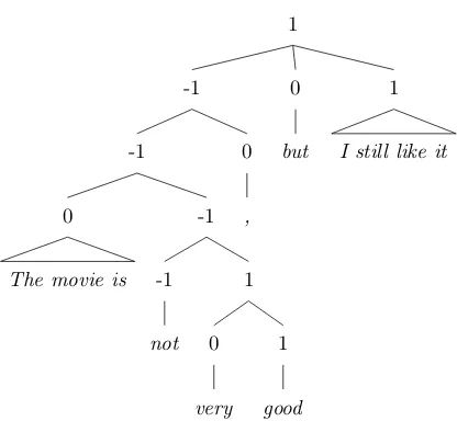
Though effective, existing neural methods do not consider explicitsentiment compositionality( Mon-tague,1974). Take the sentence “The movie is not very good, but I still like it” in Figure1as example (Dong et al.,2015), over the constituent tree, sen-timent signals can be propagated from leaf nodes to the root, going through negation, intensification and contrast according to the context. Modeling such signal channels can intuitively lead to more
∗
Work was done when the first author was visiting West-lake University. The third author is the corresponding author.
Draw tree
guiwuqiansha
March 2019
1
Introduction
1
-1
-1
0
The movie is
-1
-1
not
1
0
very 1
good 0
, 0
but
1
I still like it
[image:1.595.307.515.218.410.2]1
Figure 1: Example of sentiment composition
interpretable and reliable results. To model sen-timent composition, direct encoding of sensen-timent signals (e.g., +1/-1 or more fine-grained forms) is necessary.
To this end, we consider a neural network gram-mar with latent variables. In particular, we em-ploy a grammar as the backbone of our approach in which nonterminals represent sentiment signals and grammar rules specify sentiment compositions. In the simplest version of our approach, nonterminals are sentiment labels from SST directly, resulting in a weighted grammar. To model more fine-grained emotions (Ortony and Turner,1990), we consider a latent variable grammar (LVG,Matsuzaki et al.
(2005),Petrov et al.(2006)), which splits each non-terminal into subtypes to represent subtle sentiment signals and uses a discrete latent variable to denote the sentiment subtype of a phrase. Finally, inspired by the fact that sentiment can be modeled with a low dimensional continuous space (Mehrabian,
associates each sentiment signal with a continuous vector instead of a discrete variable.
Experiments on SST show that explicit mod-eling of sentiment composition leads to signifi-cantly improved performance over standard tree encoding, and models that learn subtle emotions as hidden variables give better results than coarse-grained models. Using a bi-attentive classifica-tion network (Peters et al., 2018) as the encoder, out final model gives the best results on SST. To our knowledge, we are the first to consider neural network grammars with latent variables for senti-ment composition. Our code will be released at
https://github.com/Ehaschia/bi-tree-lstm-crf.
2 Related Work
Phrase-level sentiment analysis Li et al.(2015) andMcCann et al.(2017) proposed sequence struc-tured models that predict the sentiment polarities of the individual phrases in a sentence indepen-dently.Zhu et al.(2015),Le and Zuidema(2015),
Tai et al.(2015) andGupta and Zhang(2018) pro-posed Tree-LSTM models to capture bottom-up dependencies between constituents for sentiment analysis. In order to support information flow bidi-rectionally over trees,Teng and Zhang(2017) intro-duced a Bi-directional Tree-LSTM model that adds a top-down component after Tree-LSTM encoding. These models handle sentiment composition im-plicitly and predict sentiment polarities only based on embeddings of current nodes. In contrast, we model sentiment explicitly.
Sentiment composition Moilanen and Pulman
(2007) introduced a seminal model for sentiment composition (Montague,1974), composed positive, negative and neutral (+1/-1/0) singles hierarchi-cally. Taboada et al. (2011) proposed a lexicon-based method for addressing sentence level contex-tual valence shifting phenomena such as negation and intensification. Choi and Cardie(2008) used a structured linear model to learn semantic composi-tionality relying on a set of manual features.Dong et al.(2015) developed a statistical parser to learn the sentiment structure of a sentence. Our method is similar in that grammars are used to model se-mantic compositionality. But we consider neural methods instead of statistical methods for senti-ment composition. Teng et al.(2016) proposed a simple weighted-sum model of introducing senti-ment lexicon features to LSTM for sentisenti-ment analy-sis. They used -2 to 2 represent sentiment polarities.
In contrast, we model sentiment subtypes with la-tent variables and combine the strength of neural encoder and hierarchical sentiment composition.
Latent Variable Grammar There has been a line of work using discrete latent variables to en-rich coarse-grained constituent labels in phrase-structure parsing (Johnson,1998;Matsuzaki et al.,
2005;Petrov et al.,2006;Petrov and Klein,2007). Our work is similar in that discrete latent variables are used to model sentiment polarities. To our knowledge, we are the first to consider modeling fine-grained sentiment signals by investigating dif-ferent types of latent variables. Recently, there has been work using continuous latent vectors for mod-eling syntactic categories (Zhao et al.,2018). We consider their grammar also in modeling sentiment polarities.
3 Baseline
We take the constituent Tree-LSTM as our baseline, which extends sequential LSTM to tree-structured network topologies. Formally, our model computes a parent representation from its two children in a Tree-LSTM:
i fl fr o g
=
σ σ σ σ
tanh
Wt
x hl hr
+bt
(1)
cp =i⊗g+fl⊗cl+fr⊗cr (2)
hp =o⊗tanh(cp) (3)
whereWt ∈R5Dh×3Dhandb
t ∈R3Dhare
train-able parameters,⊗is the Hadamard product and xrepresents the input of leaf node. Our formula-tion is a special case of theN-ary Tree-LSTM (Tai et al.,2015) withN = 2.
Existing work (Tai et al. (2015), Zhu et al.
(2015)) performs softmax classification on each node according to the state vetcorhon each node for sentiment analysis. We follow this method in our baseline model.
4 Sentiment Grammars
which model the correlation between different sen-timent labels over a tree. Depending on how a sentiment label is represented, we develop three in-creasingly complex models. In particular, the first model, which is introduced in Section4.1, uses a weighted grammar to model the first-order corre-lation between sentiment labels in a tree. It can be regarded as a PCFG model. The second model, which is introduced in Section4.2, introduces a dis-crete latent variable for a refined representation of sentiment classes. Finally, the third model, which is introduced in Section4.3, considers a continuous latent representation of sentiment classes.
4.1 Weighted Grammars
Formally, a sentiment grammar is defined as
G = (N, S,Σ, Rt, Re, Wt, We), where N =
{A, B, C, ...} is a finite set of sentiment polari-ties, S ∈ N is the start symbol, Σis a finite set of terminal symbols representing words such that
N ∩Σ =∅,Rtis the transition rule set
contain-ing production rules of the formX α where
X ∈N andα ∈N+;Reis the emission rule set
containing production rules of the formX w whereX ∈N andw∈Σ+. W
tandWe are sets
of weights indexed by production rules inRtand
Re, respectively. Different from standard formal
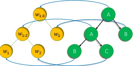
grammars, for each sentiment polarity in a parse tree our sentiment grammar invokes one emission rule to generate a string of terminals and invokes zero or one transition rule to product its child senti-ment polarities. This is similar to the behavior of hidden Markov models. Therefore, in a parse tree each non-leaf node is a sentiment polarity and is connected to exactly one leaf node which is a string of terminals. The terminals that are connected to the parent node can be obtained by concatenating the leaf nodes of its child nodes. Figure2shows an example for our sentiment grammar. In this paper, we only considerRtin the Chomsky normal form
(CNF) for clarity of presentation. However, it is straightforward to extend our formulation to the general case.
The score of a sentiment treeT conditioned on a sentencewis defined as follows:
S(T|w, K) = Y
rt∈T
Wn(rt)× Y
re∈T
We(re) (4)
where rt and re represent a transition rule and
an emission rule in sentiment parse tree T, re-spectively. We specify the transition weightsWn
with a non-negative rank-3 tensor. We compute
C B
A A
B
𝑤1 𝑤2
𝑤1:2 𝑤3
[image:3.595.310.523.66.172.2]𝑤1:3
Figure 2: Sentiment grammar example. Here yellow nodes are leaf nodes of green constituent nodes, blue
line B w1 and black lineA BC represent an
emission rule and a transition rule, respectively.
the non-negative weight of each emission rule
We(X wi:j) by applying a single layer
per-ceptronfX and an exponential function to the
neu-ral encoder state vectorhi:j representing the
con-stituentwi:j.
Sentiment grammars provides a principled way for explicitly modeling sentiment composition, and through parameterizing the emission rules with neu-ral encoders, it can take the advantage of deep learn-ing. In particular, by adding a weighted grammar on top of a tree-LSTM, our model is reminiscent of LSTM-CRF in the sequence structure.
4.2 Latent Variable Grammars
Inspired by categorical models (Ortony and Turner,
1990) which regard emotions as an overlay over a series of basic emotions, we extend our sentiment grammars with Latent Variable Grammars (LVGs;
Petrov et al.(2006)), which refine each constituent tree node with a discrete latent variables, splitting each observed sentiment polarity into finite unob-served sentiment subtypes. We refer to trees over unsplit sentiment polarities asunrefined treesand trees over sentiment subtypes asrefined trees.
Suppose that the sentiment polaritiesA,BandC
of a transition ruleABCare split intonA,nB
andnCsubtypes, respectively. The weights of the
refined transition rule can be represented by a non-negative rank-3 tensor WABC ∈ RnA×nB×nC.
Similarly, given an emission ruleA wi:j, the
weights of its refined rules by splittingAintonA
subtypes is a non-negative vectorWAwi:j ∈R
nA
calculated by an exponential function and a single layer perceptronfA:
WAwi:j = exp(fA(hi:j)) (5)
where hi:j is the vector representation of
is defined as the product of weights of all transition rules and emission rules that make up the refined parse tree, similar to Equation4. The score of an unrefined parse tree is then defined as the sum of the scores of all refined trees that are consistent with it.
Note that Weighted Grammar (WG) can be viewed as a special case of LVGs where each senti-ment polarity has one subtype.
4.3 Gaussian Mixture Latent Vector Grammars
Inspired by continuous models (Mehrabian,1980) which model emotions in a continuous low dimen-sional space, we employ Latent Vector Grammars (LVeGs) (Zhao et al., 2018) that associate each sentiment polarity with a latent vector space repre-senting the set of sentiment subtypes. We follow the idea of Gaussian Mixture LVeGs (GM-LVeGs) (Zhao et al.,2018), which uses Gaussian mixtures to model weight functions. Because Gaussian mix-tures have the nice property of being closed under product, summation, and marginalization, learning and parsing can be done efficiently using dynamic programming
In GM-LVeG, the weight function of a transition or emission ruleris defined as a Gaussian mixture withKrmixture components:
Wr(r) = Kr X
k=1
ρr,kN(r|µr,k,Σr,k) (6)
whereris the concatenation of the latent vectors representing subtypes for sentiment polarities in rule r, ρr,k > 0 is the k-th mixing weight (the
Kr mixture weights do not necessarily sum up
to 1), andN(r|µr,k,Σr,k)denotes thek-th
Gaus-sian distribution parameterized by meanµr,kand
co-variance matrix Σr,k. For an emission rule
A wi:j, all the Gaussian mixture parameters
are calculated by single layer perceptrons from the vector representationhi:j of constituentwi:j:
ρr,k = exp(fAρ,k(hi:j))
µr,k = fAµ,k(hi:j) (7) Σr,k = exp(fAΣ,k(hi:j))
For the sake of computational efficiency, we use Gaussian distributions with diagonal co-variance matrices.
4.4 Parsing
The goal of our task is to find the most probable sentiment parse treeT∗, given a sentencewand its constituency parse tree skeletonK. The polarity of the root node represents the polarity of the whole sentence, and the polarity of a constituent node is considered as the polarity of the phrase spanned by the node. Formally,T∗is defined as:
T∗ = argmax
T∈G(w,K)
P(T|w, K) (8)
where G(w, K) denotes the set of unrefined sentiment parse trees for w with skeleton K.
P(T|w, K)is defined based on the parse tree score Equation4:
P(T|w, K) = P S(T|w, K)
ˆ
T∈KS( ˆT|w, K)
. (9)
Note that unlike syntactic parsing, on SST we do not need to consider structural ambiguity, and thus resolving only rule ambiguity.
T∗ can be found using dynamic programming such as the CYK algorithm for WG. However, pars-ing becomes intractable with LVGs and LVeGs since we have to compute the score of an unre-fined parse tree by summing over all of its reunre-fined versions. We use the best performing max-rule-product decoding algorithm (Petrov et al., 2006;
Petrov and Klein,2007) for approximate parsing, which searches for the parse tree that maximizes the product of the posteriors (or expected counts) of unrefined rules in the parse tree. The detailed procedure is described below, which is based on the classic inside-outside algorithm.
For LVGs, we first use dynamic programming to recursively calculate the inside score function
sAI(a, i, j) and outside score function sAO(a, i, j)
for each sentiment polarity over each span wi:j
consistent with skeleton K using Equation 10
and Equation 11 in Table1, respectively. Simi-larly for LVeGs, we recursively calculate inside score functionsAI(a, i, j)and outside score func-tion sAO(a, i, j) in LVeG are calculated by Equa-tion13and Equation14in Table1, in which we replace the sum of discrete variables in Equation10
-11with the integral of continuous vectors. Next, using Equation12and Equation15in Table1, we calculate the score s(A BC, i, k, j) for LVG and LVeG, respectively, wherehABC, i, k, ji
represents an anchored transition rule A BC
sAI(a, i, j) = P ABC∈Rt
X
b∈N X
c∈N
WAwi:j(a) WABC(a, b, c)×s
B
I (b, i, k) sCI (c, k+ 1, j).(10)
sAO(a, i, j) = P BCA∈Rt
X
b∈N X
c∈N
WAwi:j(a) WBCA(b, c, a)×s
B
O(b, k, j)sCI (c, k, i−1)
+ P
BAC∈Rt
X
b∈N X
c∈N
WAwi:j(a) WBAC(b, a, c)×s
B
O(b, i, k) sCI (c, j+ 1, k).(11)
s(ABC, i, k, j) =X
a∈N X
b∈N X
c∈N
WABC(a, b, c)×s
A
O(a, i, j)×sBI (b, i, k)×sCI (c, k+ 1, j). (12)
sAI(a, i, j) = P ABC∈Rt
Z Z
WAwi:j(a)WABC(a,b,c)×s
B
I (b, i, k)sCI (c, k+ 1, j)dbdc(13).
sAO(a, i, j) = P BCA∈Rt
Z Z
WAwi:j(a)WBCA(b,c,a)×s
B
O(b, k, j)sCI (c, k, i−1)dbdc
+ P
BAC∈Rt
Z Z
WAwi:j(a)WBAC(b,a,c)×s
B
O(b, i, k)sCI (c, j+ 1, k)dbdc.(14)
s(ABC, i, k, j) =
Z Z Z
WABC(a,b,c)×s
A
[image:5.595.70.525.67.370.2]O(a, i, j)×sBI (b, i, k)×sCI (c, k+ 1, j)dadbdc.(15)
Table 1: Equation10-12calculate the inside score, outside score and production rule score for LVG, respectively. Equation 13-15is used for LVeG. Equation10 and Equation 13 are the inside score functions of a sentiment polarityAover its spanwi:jin the sentencew1:n. Equation11and Equation14are the outside score functions of a sentiment polarityAover a spanwi:j in the sentencew1:n. Equation12and Equation15: the production rule score function of a ruleABCwith sentiment polaritiesA,B, andCspanning wordswi:j,wi,k−1, andwk+1:j respectively. Here we use lower case lettersa,b,c . . . represent discrete subtypes of sentiment polaritiesA,B, C . . . in LVG and use bold lower case lettersa,b,c. . . represent continuous subtypes of sentiment polarities in LVeG. Note that spans such aswi:jmentioned above are all given by the skeletonKof sentencew1:n.
wk+1:j (all being consistent with skeletonK),
re-spectively. The posterior (or expected count ) of
hABC, i, k, jican be calculate as follows:
q(ABC, i, k, j) = s(A, BC, i, k, j)
sI(S,1, n)
, (16)
where sI(S,1, n)is the inside score for the start
symbolS over the whole sentencew1:n. Then we
can run CYK algorithm to identify the parse tree that maximizes the product of rule posteriors. It’s objective function is given by:
Tq∗= argmax
Tq∈G(w,K)
Y
e∈T
q(e) (17)
whereeranges over all the transition rules in the sentiment parse treeT.
Note that the equations in Table 1are tailored for our sentiment grammars and differ from their standard versions in two aspects. First, we take
into account the additional emission rules in the inside and outside computation; second, the parse tree skeleton is assumed given and hence the split pointkis prefixed in all the equations.
4.5 Learning
Given a training dataset D = {Ti,wi, Ki|i =
1. . . m} containing m samples, where Ti is the
gold sentiment parse tree for the sentencewiwith
its corresponding gold tree skeletonKi. The
dis-criminative learning objective is to minimize the negative log conditional likelihood:
L(Θ) =−log
m Y
i=1
PΘ(Ti|wi, Ki), (18)
before being back-propagated to the tree-LSTM layer.
The gradient computation for the three models involves computing expected counts of rules, which has been described in Section 4.4. For WG and LVG, the derivative of Wr, the parameter of an
unrefined production ruleris:
∂L(Θ)
∂Wr
=
m X
i=1
(EΘ[fr(t)|Ti]−EΘ[fr(t)|wi]),(19)
whereEΘ[fr(t)|Ti]denotes the expected count of
the unrefined production rulerwith respect toPΘ in the set of refined treest, which are consistent with the observed parse treeT. Similarly, we use
EΘ[fr(t)|wi]for the expectation over all
deriva-tions of the sentencewi.
For LVeG, the derivative with respect toΘr, the
parameters of the weight function Wr(r) of an
unrefined production ruleris:
∂L(Θ)
∂Θr
=
m X
i=1
Z
∂Wr(r)
∂Θr
(20)
× EΘ[fr(t)|wi]−EΘ[fr(t)|Ti]
Wr(r)
dr.
The two expectations in Equation 19and 20can be efficiently computed using the inside-outside algorithm in Table1. The derivative of the param-eters of neural encoder can be derived from the derivative of the parameters of the emission rules.
5 Experiments
To investigate the effectiveness of modeling sen-timent composition explicitly and using discrete variables or continuous vectors to model sentiment subtypes, we compare standard constituent Tree-LSTM (ConTree) with our models ConTree+WG, ConTree+LVG and ConTree+LVeG, respectively. To show the universality of our approaches, we also experiment with the combination of a state-of-the-art sequence structured model, bi-attentive classifi-cation network (BCN,Peters et al.(2018)), with our model: BCN+WG, BCN+LVG and BCN+LVeG.
5.1 Data
We use Stanford Sentiment TreeBank (SST,Socher et al.(2013)) for our experiments. Each constituent node in a phrase-structured tree is manually as-signed an integer sentiment polarity from 0 to 4, which correspond to five sentiment classes: very
negative, negative, neutral, positive and very pos-itive, respectively. The root label represents the sentiment label of the whole sentence. The con-stituent node label represents the sentiment label of the phrase it spans. We perform both binary classi-fication (-1, 1) and fine-grained classiclassi-fication (0-4), called SST-2 and SST-5, respectively. Following previous work, we use the labels of all phrases and gold-standard tree structures for training and test-ing. For binary classification, we merge all positive labels and negative labels.
5.2 Experimental Settings
Hyper-parameters For ConTree, word vectors are initialized using Glove (Pennington et al.,2014) 300-dimensional embeddings and are updated to-gether with other parameters. We set the hidden size of hidden units is 300. Adam (Kingma and Ba,2014) is used to optimize the parameters with learning rate is 0.001. We adopt Dropout after the Embedding layer with a probability of 0.5. The sentence level mini-batch size is 32. For BCN ex-periment, we follow the model setting inMcCann et al.(2017) except the sentence level mini-batch is set to 8.
5.3 Development Experiments
We use the SST development dataset to investigate different configurations of our latent variables and Gaussian mixtures. The best performing parame-ters on the development set are used in all following experiments.
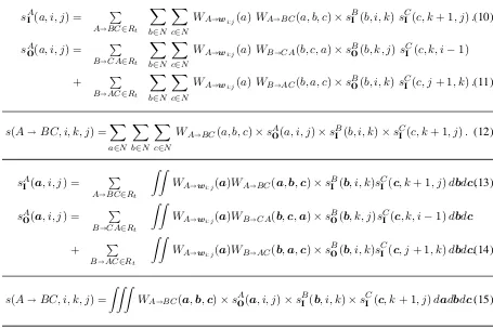
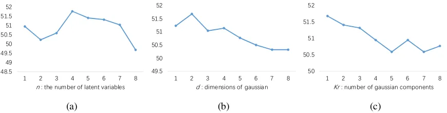
LVG subtype numbers To explore the suitable number of latent variables to model subtypes of a sentiment polarity, we evaluate our ConTree+LVG model with different number of latent variables from 1 to 8. Figure 6(a) shows that there is an upward trend while the number of hidden variables
nincreases from 1 to 4. After reaching the peak whenn= 4, the accuracy decreases as the number of latent variable continue to increase. We thus choosen= 4for remaining experiments.
48.5 49 49.5 50 50.5 51 51.5 52
1 2 3 4 5 6 7 8 n : the number of latent variables
(a)
49.5 50 50.5 51 51.5 52
1 2 3 4 5 6 7 8
d : dimensions of gaussian
(b)
50 50.5 51 51.5 52
1 2 3 4 5 6 7 8
Kr : number of gaussian components
[image:7.595.81.516.64.174.2](c)
Figure 6: Sentence level accuraicies on the development dataset. Figure (a) shows the performance of Con-Tree+LVG with different latent variables. Figure (b) and Figure (c) show the performance of ConTree+LVeG with different Gaussian dims and Gaussian mixture component numbers, respectively.
Model SST-5 Root SST-5 Phrase SST-2 Root SST-2 Phrase ConTree (Le and Zuidema,2015) 49.9 - 88.0 -ConTree (Tai et al.,2015) 51.0 - 88.0
-ConTree (Zhu et al.,2015) 50.1 - -
-ConTree (Li et al.,2015) 50.4 83.4 86.7 -ConTree (Our implementation) 51.5 82.8 89.4 86.9
ConTree + WG 51.7 83.0 89.7 88.9
ConTree + LVG4 52.2 83.2 89.8 89.1
[image:7.595.84.513.231.356.2]ConTree + LVeG 52.9 83.4 89.8 89.5
Table 2: Experimental results with constituent Tree-LSTMs.
Model SST-5 SST-2
Root Phrase Root Phrase
BCN(P) 54.7 - -
-BCN(O) 54.6 83.3 91.4 88.8 BCN+WG 55.1 83.5 91.5 90.5 BCN+LVG4 55.5 83.5 91.7 91.3 BCN+LVeG 56.0 83.5 92.1 91.6
Table 3: Experimental results with ELMo. BCN(P) is the BCN implemented byPeters et al.(2018). BCN(O) is the BCN implemented by ourselves.
LVeG Gaussian mixture component numbers
Future 6(c) shows the performance of different component numbers with fixing the Gaussian di-mension to 2. With the increase of Gaussian com-ponent number, the fine-grained sentence level ac-curacy declines slowly. The best performance is obtained when the component number Kr = 1,
which we choose for remaining experiments.
5.4 Main Results
We re-implement constituent Tree-LSTM (Con-Tree) ofTai et al.(2015) and obtain better results than their original implementation. We then in-tegrate ConTree with Weighted Grammars (Con-Tree+WG), Latent Variable Grammars with a
sub-type number of 4 (ConTree+LVG4), and Latent Variable Grammars (ConTree+LVeG), respectively. Table2 shows the experimental results for senti-ment classification on both SST-5 and SST-2 at the sentence level (Root) and all nodes (Phrase).
The performance improvement of ConTree+WG over ConTree reflects the benefit of handling sentiment composition explicitly. Particularly the phrase level binary classification task, Con-Tree+WG improves the accuracy by 2 points.
Compared with ConTree+WG, ConTree+LVG4 improves the fine-grained sentence level accuracy by 0.5 point, which demonstrates the effectiveness of modeling the sentiment subtypes with discrete variables. Similarly, incorporating Latent Vector Grammar into the constituent Tree-LSTM, the per-formance improvements, especially on the sentence level SST-5, demonstrate the effectiveness of mod-eling sentiment subtypes with continuous vectors. The performance improvements of ConTree+LVeG over ConTree+LVG4 show the advantage of infinite subtypes over finite subtypes.
0 0.5 1 1.5 2 2.5 3
words 1<=h<5 5<=h<10 h>=10 WG
[image:8.595.309.522.65.257.2]LVG4 LVeG
Figure 7: Changes in phrase level 5-class accuracies of our methods over ConTree.
with character convolutions on a large-scale cor-pus (ELMo) and reported an accuracy of 54.7 on sentence-level SST-5. For fair comparison, we also augment our model with ELMo. Table 3
shows that our methods beat the baseline on ev-ery task. BCN+WG improves accuracies on all task slightly by modeling sentiment composition explicitly. The obvious promotion of BCN+LVG4 and BCN+LVeG shows that explicitly modeling sentiment composition with fine-grained sentiment subtypes is useful. Particularly, BCN+LVeG im-proves the sentence level classification accurracies by 1.4 points (fine-grained) and 0.7 points (binary) compared to BCN (our implementation), respec-tively. To our knowledge, we achieve the best re-sults on the SST dataset.
5.5 Analysis
We make further analysis of our methods based on the constituent Tree-LSTM model. In the follow-ing, using WG, LVG and LVeG denote our three methods, respectively.
Impact on words and phrases Figure7shows the accuracy improvements over ConTree on phrases of different heights. Here the height h
of a phrase in parse tree is defined as the distance between its corresponding constituent node and the deepest leaf node in its subtree. The improvement of our methods on word nodes, whose height is 0, is small because neural networks and word embed-dings can already capture the emotion of words. In fact, the accuracy of ConTree on word nodes reaches 98.1%. As the height increases, the per-formance of our methods increase, expect for the accuracies of WG whenh ≥10since the coarse-grained sentiment representation is far difficulty for handling too many sentiment compositions over the tree structure. The performance improvements of
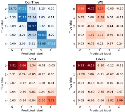
Figure 8: Top left is the normalized confusion matrix on the 5-class phrase level test dataset for ConTree. The others are the performance changs of our model over ConTree. Value in each cell is written with a unit of×10−2
LVG4 and LVeG whenh≥10show modeling fine-grained sentiment signals can represent sentiment of higher phrases better.
Impact on sentiment polarities Figure8shows the performance changes of our models over Con-Tree on different sentiment polarities. The accuracy of every sentiment polarity on WG over ConTree improves slightly. Compared with ConTree, the accuracies of LVG4 and LVeG on extreme sen-timents (the strong negative and strong positive sentiments) receive significant improvement. In addition, the proportion of extreme emotions mis-classified as weak emotions (the negative and posi-tive sentiments) drops dramatically. It indicates that LVG4 and LVeG can capture the subtle difference between extreme sentiments and weak sentiments by modeling sentiment subtypes explicitly.
[image:8.595.74.285.66.179.2]Extremely dumb . Extremely dumb
Extremely boring .
Extremely boring boring
A real clunker .
clunker . Ridiculous .
is bad . is bad
bad It 's painful .
hate this movie
hate
awful and
A dreadful live-action movie .
dreadful A very bad sign .
stupider
[image:9.595.77.252.77.178.2]Boring bloody mess .
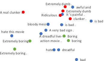
Figure 9: Visualization of correlation of phrases not longer than 5 in the strong negative sentiment space
“stupider” and “Ridiculous” (red dots) are mainly located at the top right and negative emotions with no special emotional tendency such as “hate” and “bad” (blue dots) are evenly distributed throughout the space. This demonstrates that LVeG can capture sentiment subtypes.
6 Conclusion
We presented a range of sentiment grammars for using neural networks to model sentiment com-position explicitly, and empirically showed that explicit modeling of sentiment composition with fine-grained sentiment subtypes gives better perfor-mance compared to state-of-the-art neural network models in sentiment analysis. By using EMLo em-beddings, our final model improves fine-grained accuracies by 1.3 points compare to the current best result.
Acknowledgments
This work was supported by the Major Program of Science and Technology Commission Shang-hai Municipal (17JC1404102) and NSFC (No. 61572245) . We would like to thank the anony-mous reviewers for their careful reading and useful comments.
References
Yejin Choi and Claire Cardie. 2008. Learning with
compositional semantics as structural inference for subsentential sentiment analysis. InProceedings of the conference on empirical methods in natural lan-guage processing, pages 793–801. Association for Computational Linguistics.
Li Dong, Furu Wei, Shujie Liu, Ming Zhou, and Ke Xu. 2015. A statistical parsing framework for sentiment classification. Computational Linguistics, 41(2):293–336.
Amulya Gupta and Zhu Zhang. 2018. To attend or not to attend: A case study on syntactic structures for semantic relatedness. InProceedings of the 56th An-nual Meeting of the Association for Computational Linguistics (Volume 1: Long Papers), volume 1, pages 2116–2125.
Mark Johnson. 1998. Pcfg models of linguistic tree rep-resentations. Computational Linguistics, 24(4):613– 632.
Diederik Kingma and Jimmy Ba. 2014. Adam: A
method for stochastic optimization. International Conference on Learning Representations.
Phong Le and Willem Zuidema. 2015. Compositional
distributional semantics with long short term mem-ory. InProceedings of the Fourth Joint Conference on Lexical and Computational Semantics, pages 10– 19. Association for Computational Linguistics.
Jiwei Li, Thang Luong, Dan Jurafsky, and Eduard Hovy. 2015. When are tree structures necessary for deep learning of representations? InProceedings of the 2015 Conference on Empirical Methods in Nat-ural Language Processing, pages 2304–2314. Asso-ciation for Computational Linguistics.
Takuya Matsuzaki, Yusuke Miyao, and Jun’ichi Tsu-jii. 2005. Probabilistic cfg with latent annotations. InProceedings of the 43rd annual meeting on Asso-ciation for Computational Linguistics, pages 75–82. Association for Computational Linguistics.
Bryan McCann, James Bradbury, Caiming Xiong, and Richard Socher. 2017. Learned in translation: Con-textualized word vectors. InAdvances in Neural In-formation Processing Systems, pages 6294–6305.
Albert Mehrabian. 1980. Basic dimensions for a gen-eral psychological theory: Implications for person-ality, social, environmental, and developmental stud-ies. Oelgeschlager, Gunn & Hain Cambridge, MA.
Karo Moilanen and Stephen Pulman. 2007. Sentiment composition. InProceedings of RANLP, volume 7, pages 378–382.
Richard Montague. 1974. Formal Philosophy;
Se-lected Papers of Richard Montague. New Haven: Yale University Press.
Andrew Ortony and Terence J. Turner. 1990. What’s basic about basic emotions? Psychological Review, 97(3):315–331.
Jeffrey Pennington, Richard Socher, and Christopher Manning. 2014. Glove: Global vectors for word rep-resentation. InProceedings of the 2014 conference on empirical methods in natural language process-ing (EMNLP), pages 1532–1543.
of the North American Chapter of the Association for Computational Linguistics: Human Language Technologies, Volume 1 (Long Papers), pages 2227– 2237. Association for Computational Linguistics.
Slav Petrov, Leon Barrett, Romain Thibaux, and Dan Klein. 2006. Learning accurate, compact, and inter-pretable tree annotation. InProceedings of the 21st International Conference on Computational Linguis-tics and the 44th annual meeting of the Association for Computational Linguistics, pages 433–440. As-sociation for Computational Linguistics.
Slav Petrov and Dan Klein. 2007. Improved inference for unlexicalized parsing. InHuman Language Tech-nologies 2007: The Conference of the North Amer-ican Chapter of the Association for Computational Linguistics; Proceedings of the Main Conference, pages 404–411.
Richard Socher, Alex Perelygin, Jean Wu, Jason Chuang, Christopher D Manning, Andrew Ng, and
Christopher Potts. 2013. Recursive deep models
for semantic compositionality over a sentiment
tree-bank. In Proceedings of the 2013 conference on
empirical methods in natural language processing, pages 1631–1642.
Maite Taboada, Julian Brooke, Milan Tofiloski, Kim-berly Voll, and Manfred Stede. 2011. Lexicon-based methods for sentiment analysis. Computational lin-guistics, 37(2):267–307.
Kai Sheng Tai, Richard Socher, and Christopher D. Manning. 2015. Improved semantic representations from tree-structured long short-term memory net-works. In Proceedings of the 53rd Annual Meet-ing of the Association for Computational LMeet-inguis- Linguis-tics and the 7th International Joint Conference on Natural Language Processing (Volume 1: Long Pa-pers), pages 1556–1566. Association for Computa-tional Linguistics.
Zhiyang Teng, Duy Tin Vo, and Yue Zhang. 2016. Context-sensitive lexicon features for neural senti-ment analysis. InProceedings of the 2016 Confer-ence on Empirical Methods in Natural Language Processing, pages 1629–1638.
Zhiyang Teng and Yue Zhang. 2017. Head-lexicalized bidirectional tree lstms. Transactions of the Associ-ation for ComputAssoci-ational Linguistics, 5:163–177.
Yanpeng Zhao, Liwen Zhang, and Kewei Tu. 2018.
Gaussian mixture latent vector grammars. In Pro-ceedings of the 56th Annual Meeting of the Associa-tion for ComputaAssocia-tional Linguistics (Volume 1: Long Papers), pages 1181–1189. Association for Compu-tational Linguistics.
Xiaodan Zhu, Parinaz Sobihani, and Hongyu Guo. 2015. Long short-term memory over recursive
struc-tures. In International Conference on Machine