ABSTRACT
NAGARAJAN, RAJESH. An Industrial Application of the 2-Dimensional Finite Bin Packing Problem. (Under the direction of Professor Robert. B. Handfield).
The 2-Dimensional Finite Bin Packing Problem is a NP hard problem with it being observed in many of the process industries like woodcutting, textile manufacturing and steel industry. Here the scenario is a fiberglass mesh manufacturing industry, whose prime objective is to reduce material wastages due to cutting. We evaluate a few exact methods and a few heuristic techniques, which have been proposed to solve this problem. We further select Finite Best-Strip algorithm for implementation. We make modification to that technique to handle guillotine constraints. An after effect of this technique is observed in order tracking, which is reduced using k-way graph partitioning technique. The problem is tested for its performance by using datasets provided by the company. The results obtained are compared with the actual scenario. The experimental results show that this technique performs much better than the currently used technique and also a much better upper bound on the solution is observed when compared to previously known upper bounds for problems of these types. We also discuss on the future scope and enhancements possible for this technique to obtain better results.
BIOGRAPHY
Rajesh Nagarajan, born on the New Year eve of 1977 in the beautiful city of Belgaum in the state of Karnataka, India, completed his schooling from the city of Mysore, India. He obtained his Bachelors of Engineering degree in Mechanical Engineering from Bangalore University. Before joining the Operations Research Program at North Carolina State University he worked as a “Production Planning Engineer” for a year at John Fowler (India) Pvt. Ltd in Bangalore, India.
During his graduate studies at North Carolina State University he undertook course work in Operations Research and Supply Chain Management. He worked on various industry relate problems in the area of supply chain management under Dr. Robert Handfield. During his graduate studies he did an internship at Defense Group Inc. as a “Research Analyst”. His areas of interests include supply chain management, discrete optimization and discrete event simulation.
ACKNOWLEDGEMENTS
First and foremost I would like to thank my parents Mrs. Mangala Nagarajan and Mr. Nagarajan whose encouragement and support has helped me in my success. I would also like to thank my advisor Dr. Robert Handfield for his valuable guidance and support. I am grateful to my committee members Dr. Yahya Fathi and Dr. Ralph Smith for their support and encouragement.
I am also grateful to the support by my other family members Mohan, Jyothi and Madhu. I would also like to mention my friends Divya, Pooja, Archana, Girish, Bobby, Sai, Manish, Sachin, Prashant, Virendra, Ambarish and Mohan for their valuable company, which I shall cherish forever.
TABLE OF CONTENTS
LIST OF FIGURES ... vi
LIST OF TABLES...vii
1
Introduction... 1
1.1 SCENARIO... 1 1.1.1 Company Background ... 11.1.2 Sales and Distribution... 2
1.2 PRODUCTION TECHNOLOGY... 3
1.3 MANUFACTURING PROCESS: ... 3
1.4 DESCRIPTION OF THE PROBLEM... 4
1.4.1 2-Dimensional finite bin packing problem... 5
1.4.2 Guillotine cutting... 6
2
Related research ... 7
2.1 EXACT SOLUTION... 7
2.2 HEURISTIC TECHNIQUES... 8
2.2.1 Finite Next-Fit Heuristic ... 8
2.2.2 Finite First-Fit Heuristic... 8
2.2.3 Finite Bottom-Left Heuristic ... 9
2.2.4 Finite Best-Strip Heuristic ... 9
2.2.5 A New Finite Best-strip Heuristic ... 10
3
Solution Implementation... 12
3.1 DATA PRE-PROCESSING... 12
3.1.2 Order Sorting ... 13
3.2 MODIFIED FINITE BEST-STRIP HEURISTIC... 13
3.2.1 Defining Levels... 13
3.2.2 Best-strip packing... 13
3.3 REGROUPING USING K-WAY GRAPH PARTITIONING APPROACH... 15
3.3.1 Initial Partitioning Phase... 16
3.3.2 Value of graph... 16 3.3.3 Neighborhood Structure... 16 3.3.4 Search Procedure... 17 3.3.5 Objective Function ... 18 3.4 SURPLUS ESTIMATION... 18 3.5 PSEUDO CODE... 19
4
Results and Observation ... 21
4.1 COMPUTATION SETUP... 21
4.2 PERFORMANCE OF MODIFIED FINITE BEST-STRIP HEURISTIC... 21
4.2.1 Packing Efficiency... 21
4.2.2 Upper bound... 22
4.3 PERFORMANCE OF K-WAY GRAPH PARTITIONING ALGORITHM... 23
4.4 EFFECT OF SURPLUS ESTIMATION... 24
4.5 CONCLUDING REMARKS... 25
5
Summary and future scope of work ... 26
6
References... 28
LIST OF FIGURES
Figure 1: Schematic representation of the Manufacturing Process ... 3
Figure 2: Guillotine cutting pattern ... 6
Figure 3: Order Break-up Process ... 12
Figure 4: Packing process in Modified Finite Best-Fit packing heuristic ... 15
Figure 5: Process for Surplus Estimation ... 18
Figure 6: Pseudo Code for Modified Finite Best-Strip Heuristic ... 20
Figure 7: Effect of Surplus Allowance ... 24
Figure 8: Screen image of Input Form ... 29
LIST OF TABLES
Table 1: Summary of results for Modified Finite Best-Fit Heuristic... 22 Table 2: Performance Analysis of k-way Graph Partitioning Algorithm ... 23 Table 3: Performance Analysis of Existing System Vs. New developed System... 25
1 Introduction
1.1 Scenario
In the 21st century the usage of fiberglass in day-to-day life has increased multifold. To cater to this need is CCX Inc a company with product base in 53 countries and its head office located in Charlotte, North Carolina.
1.1.1 Company Background
CCX1 Inc is a conglomeration of three independent successful companies viz., Hanover Wire Cloth, Braeburn Alloy Steel and CCX Fiberglass Products. Each of these companies is very successful in their respective markets. Their product ranges include screens to protect from insects, exterior insulation finishing system, concrete re-enforcement meshes and self-adhesive drywall tapes.
1.1.1.1 Hanover Wire Cloth
Hanover wire cloth established in 1903, is a leading producer of woven metallic and non-metallic products and Industrial fabrics. They operate with two weaving facilities with area of more than 780,000 square feet. Their major product lines are
• Star Brand® Insect Screening • Liquid Filtration Mesh Products • Wall-Span® Fiberglass Drywall Tape
• Concrete Reinforcement and Roofing Fabrics
• Stucco Reinforcement Mesh
• Fine Wire
• Steel Forging and Rolled Products
1
1.1.1.2 Braeburn Alloy Steel
Braeburn Alloy Steel established in 1897, and owned by CCX for nearly a half century is a fully integrated manufacturer and distributor of specialty steel bars. Braeburn Alloy Steel offers processing capabilities for a complete range of metal alloys, including titanium, refractory metals, high-nickel alloys, and stainless, tool steel, carbon steel, and alloy steel. Braeburn has been particularly successful in processing difficult-to-work materials such as high-nickel or cobalt alloys and titanium.
1.1.1.3 CCX Fiberglass Products
CCX Fiberglass Products, established in July 1989 is a leading manufacturer of scrim fabrics, coated and uncoated fiberglass and polyester mesh products including insect screening, self-adhesive drywall tapes2, concrete reinforcement mesh, roofing scrims and Exterior Insulation Facing Systems (EIFS) reinforcement mesh. Also CCX Fiberglass Products supplies fiberglass meshes to its sister company Hanover Wire Cloth. CCX Fiberglass Products operates from a 340,000 square foot in Walterboro, SC.
1.1.2 Sales and Distribution
CCX Inc do not sell their products directly to customers, rather are sold to general contractors, building product distributors, exterior insulation facing systems installers, original equipment manufacturers, converters, laminators, hardware stores and home centers. The products are sold through a national network of building product distributors directed by their facility's sales and marketing staff.
Here our matter of interest is in CCX Fiberglass Products. Our area of concentration is manufacturing of fiberglass and polyester mesh products. It was during their manufacturing that it was observed that they produce considerable amount of wastage in
2
material. Primarily this was due to wastage produced during cutting of the meshes. Hence was derived the objective to develop an efficient cutting pattern to reduce the wastages.
The cutting problems are predominant in many of the process industries like wood industry, textile industry, steel industry etc. Everywhere the main objective is to come up with an efficient cutting pattern to minimize wastages. The problem considered as a part of this thesis is highly oriented to the scenario at CCX Inc.
1.2 Production Technology
CCX Fiberglass Products uses state of the art machines and equipments during its manufacturing process that helps them provide high quality products. Their new line of equipments include a state of the art tentering unit which allows for higher productivity and increased capacity and a I-Tex tm System for the weaving operation. The I-Tex System is an automated fabric inspection system, which can detect defects as small as 0.5 mm on fabric widths up to 330 cm and at speeds that reach 100 meters per minute. This technology adds a whole new dimension in improving quality, performance and enhanced customer satisfaction.
1.3 Manufacturing Process:
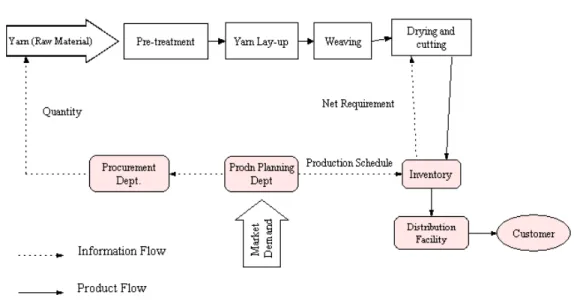
A schematic representation of the manufacturing process at CCX Inc is shown in Figure 1.
Step1: The market demand when received by the Production Planning Department is
processed to generate a Material Requirement Plan (MRP) and Production Schedule.
Step2: The raw material purchased by the Procurement Department, which is fiberglass
yarn, is subjected to pre-treatment. The input yarn is classified into two types, which is based on color.
1. Charcoal 2. Gray
Step3: Pre-treated yarn bobbins are spun onto a roll. The rolls are then fed onto the
weaving machines or looms. The looms are classified based on 1. Speed of the machine
2. Maximum width of the incoming roll that the machine can take.
Step4: The woven fabric is subject to drying. The fabric is cut to required length, which
is based on “net material requirement” generated after inventory check. Wastage produced during cutting is disposed and fabric is packed and shipped to customer.
1.4 Description of the problem
The targeted area is the Weaving Cost Center. The weaving department maintains several sets of looms, which are grouped on capacities in width (inches) and speed (square feet/min). Because of the machine constraints, the fabric is produced only on certain widths. But the market demand has varying lengths and varying widths3.
It has been observed in the past that in order to maximize machine utilization, all the machines have to be loaded to the maximum possible width. And for each loom set there
3 The machine width is designed to accommodate all the demand. (W
is a cost ($/square feet) associated in running each of the individual widths and width combinations. So for the standardized fabric woven by the weaving machines (width ‘W’ and length ‘L’) we have to come up with a cutting sequence to cut smaller pieces (width ‘w’ and length ‘l’), which would maximize machine utilization and minimize material wastage costs. This problem is very similar to a 2-dimensional finite bin-packing problem.
1.4.1 2-Dimensional finite bin packing problem
In a 2D finite bin-packing problem [1], we are given ‘n’ number of rectangular pieces. These pieces have to be cut from a larger number of uniform rectangular pieces (which are called as finite bins) with height H4 and width W. The characteristics of each of the pieces are as follows:
1. Each piece p∈P=
{
1,....,n}
2. Height of each piece is defined by hp ≤H
3. Width of each piece is defined by wp ≤W
4. The height and width cannot be reversed
The 2D finite bin-packing problem (2D FBPP) is a generalized case of 1D bin-packing problem (which is a NP-hard problem). In a 1D bin-packing problem (1D BPP) we have infinite number of bins of capacity W and n items to be placed into the bins. Each item is characterized by its weight , which is to be fitted into minimum number of bins. Since 1D BPP is a NP-hard problem and 2D FBPP being a generalized version of it, we can thus say that 2D FBPP is a NP-hard problem in strong sense.
j w
The 2D FBPP when talked about in general sense, is always assumed to have no restriction on the cutting patterns i.e., guillotine-cutting constraint is not considered. However here there is a constraint on the type of cutting possible, thus we have to impose the guillotine cutting constraint.
4
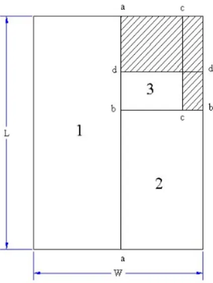
1.4.2 Guillotine cutting
Figure 2: Guillotine cutting pattern
On a rectangular piece if a cut has to be made from one edge to the opposite edge, then such a cut is termed as “Guillotine Cut” [2]. Here there is an additional constraint to the above mentioned guillotine cutting. Any piece has to be first cut across the length. The cutting pattern is shown sequentially in Figure 2.
2 Related research
2.1 Exact Solution
An exact solution to the 2D-BPP was proposed by Martello et. al [1]. This method used a combination of branch and bound algorithm and heuristic algorithms to obtain the exact solution of 2D-BPP.
This algorithm adopts a nested branching scheme. The decision tree is divided into two sections viz. outer branch decision tree and inner branch decision tree.
Outer Branch Decision Tree: In this tree at each decision-node, a piece k is assigned to
a bin. The feasibility of such an assignment is done primarily by estimating the Lower Bound ‘L ’5 for the current instance. If , then assignment is not possible, thus backtracking has to be performed. Else heuristic algorithms like Finite First-Fit (FFF) or the Finite Best-Fit (FBF) is applied to the current instance of the problem. Even then if a feasible assignment is not found, then the control is passed to the Inner Branch Decision Tree, else the search continues.
1 >
L
Inner Branch Decision Tree: The non-feasible set from the outer decision tree is primarily checked for existence of such a feasible set at all by the Inner Branch Decision
Tree. If yes then search continues in the Outer Branch Decision Tree, else a backtracking
occurs.
However here, with the help of enumerative algorithms, exact solutions for problems with up to 120 pieces are defined. With higher number of pieces, the computation time is estimated to be very high.
5
2.2 Heuristic Techniques
Various heuristic algorithms have been proposed to solve the 2D-FBPP. Berkey et. al [3]. Most of the heuristic methods proposed are constructive methods and solve the problems assuming the bins with finite capacity. On an average the upper bound on the number of pieces that could be packed per bin was observed to be about 3.65.
All of the algorithms described below use a level-oriented packing approach, wherein the rectangular pieces are placed on the bottom-left most level. The initial level is the bottom of the bin. The next level is defined from the maximum height of all the pieces in the previous level. Height of each level is the distance of that level from the bottom of the bin.
2.2.1 Finite Next-Fit Heuristic
The finite next-fit heuristic has been proven to have the fastest computation time with when compared to other heuristic algorithms. But the quality of the solution obtained is relatively poor. The working of the heuristic is as described in the following steps.
) (n
O
1. The rectangular pieces are initially pre-sorted on their decreasing order of height.
2. The pieces are placed in the bin using the bottom left approach.
3. If the piece doesn’t fit then the bin is closed and a new bin is assigned.
4. At any point of time there is only one bin in the bin-list.
2.2.2 Finite First-Fit Heuristic
The finite first-fit heuristic is a modification over finite next-fit heuristic. The
computation time is . In this heuristic all the bins created are maintained in the
bin-list. Working of this heuristic is described as follows:
)
( 2
n O
1. The rectangular pieces are initially pre-sorted on their decreasing order of height.
2. Each piece is packed by beginning to search from the first created bin, checking
If the piece does not fit, then the search is performed on the next bin in the bin-list. This search terminates if successful packing is possible, else continues till all the bins in the
bin-list are exhausted. The unpacked piece is then assigned to a new bin.
2.2.3 Finite Bottom-Left Heuristic
The Finite Bottom-Left Heuristic uses the same bottom-left approach as mentioned above. The functioning of this algorithm is described below.
1. The rectangular pieces are initially pre-sorted on their decreasing order of height.
2. The rectangular piece is checked for packing into the bottom-left most position
for packing.
3. If no such bin is available then a new bin is created.
4. The unused area when enclosed by rectangular pieces on all the four sides is
called as sub-hole of the bin.
The search for possible packing location of the pieces also includes searching the
sub-holes. However from Chazelle [4] the time consumed for an exhaustive search of all the sub-holes in the Bottom-Left bin-packing approach is estimated to be O(n2).
2.2.4 Finite Best-Strip Heuristic
The finite best-strip is one of the most widely used algorithms for 2D-FBPP. This algorithm when implemented using binary search-tree data structure, is estimated to
consume time of O(nlogn). The functioning of the algorithm is as follows:
1. The rectangular pieces are initially pre-sorted on their decreasing order of height.
2. The first piece is placed in the bottom-left most position of the bin. Here initially
an open-ended strip is used to pack all the pieces.
3. The next strip selected for packing is the one whose packing would result in a
minimum remaining horizontal area. This is termed as best-fit approach.
4. Height of each level is defined by maximum height of any piece in that level.
2.2.5 A New Finite Best-strip Heuristic
The new finite best-strip heuristic has a small variation over the finite best-strip heuristic. In the best-fit approach, instead of progressing with an objective of minimizing horizontal area, the objective can be minimization of both horizontal and vertical area, thus improving the packing efficiency. This heuristic has been used to solve the problem considered in this work. Details about implementation of this heuristic is explained in the next section.
During the implementation it was observed that due to the capacity constraint on the bin size, the order size has to be split. For e.g. If the demand is for a length of 22,000 Yards and width 50” and the bin width is 100” and length is 5,000 Yards, the demand has to be broken down into 4 orders of 5,000 Yards and 1 order of 2,000 Yards. And because of the nature of this heuristic, the orders tend to be displaced into multiple bins and in turn these bins could be allocated to different machines. Due to this, tracking of orders becomes difficult. So we have to come up with a re-grouping heuristic, which would reduce the displacement, thus reducing the magnitude of the tracking problem. There are ‘n’ bins to be grouped among ‘k’ bins. This is a scenario for a k-way graph-partitioning problem.
2.2.5.1 K-way graph-partitioning problem
Graph partitioning is primarily used to schedule tasks to be executed in parallel and to minimize communication between groups. It is defined as partitioning of a graph
containing ‘ ’ vertices into ‘k’ equal partitions, such that the connections between
vertices across the partitions are minimized.
N
Let graph G=(N,E,WN,WE) (1)
Where, N → Set of nodes. N =(N1,N2,...,Nk)
E → Set of edges connecting to nodes (i, j)
→ Non-negative weight of each node.
N W
→ Non-negative weight of each edge.
E
W
Partition Balancing: Sums of weights ‘W ’ of the nodes ‘n’ in each ‘ ’ is approximately equal.
n Ni
Minimize interconnection: Sum of weights of edges ‘W ’ which connects between nodes
in different ‘ ’ and ‘ ’ combinations should be minimized.
e
i
3 Solution Implementation
In this chapter details about implementation of the Modified Finite Best-Fit Heuristic technique to solve the current problem is given. We start with description of data pre-processing, modified finite Best-Fit Heuristic packing and re-grouping of bins using graph-partitioning approach. Also details about surplus estimation, pseudo-code for modified finite Best-Fit Heuristic and K-way graph partitioning is included.
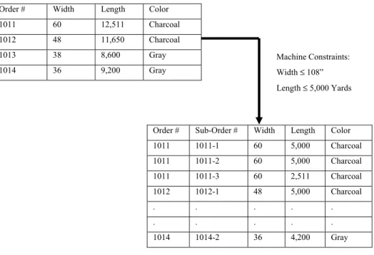
3.1 Data Pre-processing
3.1.1 Order Break-up
The net requirement as estimated by the planning department is inputted into the system.
The orders are broken down into sub-orders6, so that each sub-order meets the capacity
constraint of the machines. The table below explains the same procedure.
Order # Width Length Color
1011 60 12,511 Charcoal 1012 48 11,650 Charcoal 1013 38 8,600 Gray 1014 36 9,200 Gray Machine Constraints: Width ≤ 108” Length ≤ 5,000 Yards
Order # Sub-Order # Width Length Color 1011 1011-1 60 5,000 Charcoal 1011 1011-2 60 5,000 Charcoal 1011 1011-3 60 2,511 Charcoal 1012 1012-1 48 5,000 Charcoal . . . . . . . . . . 1014 1014-2 36 4,200 Gray
Figure 3: Order Break-up Process
6
3.1.2 Order Sorting
The sub-orders are initially divided into groups by color. Each of these groups are initially sorted in non-decreasing order of their length and then sorted in non-decreasing order of width.
3.2 Modified Finite Best-Strip Heuristic
3.2.1 Defining Levels
The initial level starts at the bottom of the bin and is termed as level 0. The height of each level is defined by height of the single largest piece in the current level. Also this marks the beginning of next level. The height of each level can be expressed as
(2) ) ,...., , max( 1,k 2,k j,k k h h h H = → height of level k. k H → height of j k j h, th piece in kth level. 3.2.2 Best-strip packing
An open-ended strip, which has constraint on its width, is considered. The width of each bin is driven by the capacity of each weaving machine. The steps below explain the best-strip packing procedure. A pseudo code for the same is described later in this chapter.
Step 1: The first piece from the pre-sorted orders list is placed at the bottom left corner of the bin. The initial level is marked level 0. The picking of the pieces from the list is done sequentially. Since the pieces are sorted on non-increasing order of length, it is evident that the first piece to be placed shall have the maximum height with respect to the following pieces. So effectively the first piece determines the height of the level. The position of each piece is represented by a 3D-array. Position of
piece ‘i’ is equal to , where p represents level, q represents horizontal
position, and r represents vertical position. The initial position starts with (0,0,0). The position of the first piece is represented as (0,1,1).
) , ,
Step2: For filling up the remaining area in the current level, again a sequential search from the pre-sorted orders list is done. The piece with the best possible fit along its width is considered. If the search results in multiple orders, which would fit this requirement, then selecting the piece having maximum area breaks the tie.
Step3: The procedure repeats till no piece exists, which would fit into remaining width.
Step4: A multi-layer stacking procedure is adopted if h where, q>1. In
words this means if the height of the pieces adjacent to the 1 ) 1 , 1 , ( ) 1 , , (pq <h p st
piece is less than
height of the 1st piece, then multi-layer stacking procedure is adopted.
Multi-layer stacking procedure: The procedure is similar to best-fit packing approach, but for the following constraints.
Constraint 1: This procedure is valid for packing pieces whose position is given by(p,q,r), where q > 1 and r > 1.
Constraint 2: Constraint on width7 is given by
) 1 , , ( ) , , (pqr w pq w ≤ , where r>1 and q>1.
Constraint 3: Constraint on height is given by ) ( ( ,1,1) ( , ,1) ) , , (pqr hp hpq h ≤ − , where r>1 and q>1.
Step5: When no more packing is possible in the current level, then the level is closed and a new level is created above this level and the procedure is repeated for all the sub-orders.
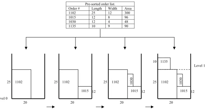
Figure 4 shows an example explaining the above-mentioned procedure.
7
Pre-sorted order list.
Order # Length Width Area 1102 25 12 300 1015 12 8 96 1030 12 4 48 1135 10 9 90 10 1135 Level 1 1030 1102 25 25 1102 25 1102 25 1102 1030 1015 12 1015 12 1015 12 Level 0 20 20 20 20
Figure 4: Packing process in Modified Finite Best-Fit packing heuristic
Step6: After packing all the pieces into the open-ended strip, then each of these pieces have to be packed into a finite bin. Each level is now considered as a rectangular piece, which is to be fitted into ‘p’ such bins. The best-fit packing approach is repeated to fill up these finite bins. The height of each bin is constrained by the machine capacity and width of each bin is similar to that of the open-ended strip. If a bin is filled to its capacity, then a new bin is created to facilitate the remaining bins. Packing of all the rectangular pieces into finite bins terminates the best-strip bin-packing algorithm.
3.3 Regrouping using k-way graph partitioning approach
During the finite best-strip packing approach, it was observed that as the orders are broken down into sub-orders and then re-sorted, the orders get spread out into different
bins. These bins8 have to be processed on weaving machines. If each order is spread out on different machines than tracking becomes a considerable issue. If the number of bins > number of machines, then multiple bins have to be scheduled on a single machine. Thus we have to come up with a scheduling sequence by which a single order can be scheduled on as minimum number of machines as possible. This problem is similar to a k-way graph-partitioning problem, wherein we have ‘k’ different partitions (machines) on which ‘n’ vertices (bins) have to be grouped (scheduled).
3.3.1 Initial Partitioning Phase
The domain is initially divided into ‘k’ phases (which is equal to the number of machines). In the beginning the bins are randomly but uniformly distributed among all the ‘k’ phases.
3.3.2 Value of graph
For every partition the number of distinctive order numbers that it contains determines its value. This value when summed up over all the partitions determines the value of the graph.
For e.g. consider a graph with 2 partitions with each containing the following order
numbers. P1 = {2,2,4,6,3,2,7,8}; P2 = {4,4,6,9,12,12,14,7}. The number of distinctive
order numbers for P1 is 5 and for P2 is 6. Thus the value of the graph is 11.
3.3.3 Neighborhood Structure
All Graphs G’ which can be obtained by moving one vertex (bin) from a partition ‘i’ to any partition ‘j’, where i≠j, forms the neighborhood of graph G. The size of the
neighborhood is given by ( n
k−1)
Where, k → number of partitions in the graph
n → number of vertices in the graph
8
3.3.4 Search Procedure
Initially all the partitions are numbered. Beginning with the 1st partition the search is
made. Any random node is picked and is placed into another partition. This forms the new solution. However this procedure tends to loose the load balancing in the graph. To compensate this a penalty function is associated with adding any new vertex to a particular partition. The penalty function ‘P’ for a partition ‘i’ is however defined as follows. 2 − = k n S Pi α i (3) Where,
1) α → Compensating factor defined between 0 and 1. This factor controls the
degree of acceptable imbalance in the graph. Higher the value more is the graph balanced.
2) Si → Existing number of bins in the current partition
3) n → total # of vertices in the entire graph
4) k → total # of partitions in the graph
It can be observed that the term
k n
determines the average number of bins per partition.
For equal partition Si =
k n
, thus making the penalty 0 and increases to the square power with any variation. However this increase is controlled by the compensating factor α.
3.3.5 Objective Function
The objective is to minimize order displacement and at the same time maintain the balance in the partition. This can however be expressed as
∑ + = = k i i P T Z MinZ 1 : (4) Where,
1) T → Value of the graph
2) Pi → Penalty cost for partition ‘i’
3) k → total # of partitions in the graph
For every new graph, Z’ is computed. If Z’≤ Z, Z=Z’, else the new solution is discarded
and search continues.
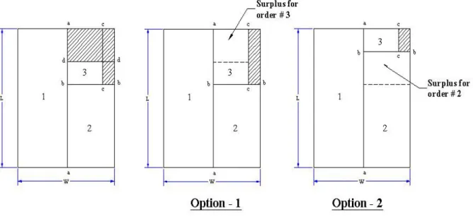
3.4 Surplus Estimation
During material processing, the other method to reduce wastage is surplus production. If instead of producing wastage, extra volume production were allowed, then there would be a considerable reduction in wastage. Figure 5 indicates reduction in wastage with surplus production.
This feature has been incorporated into the algorithm. The effectiveness of the tool can be observed in the results, which is discussed in detail in the next chapter.
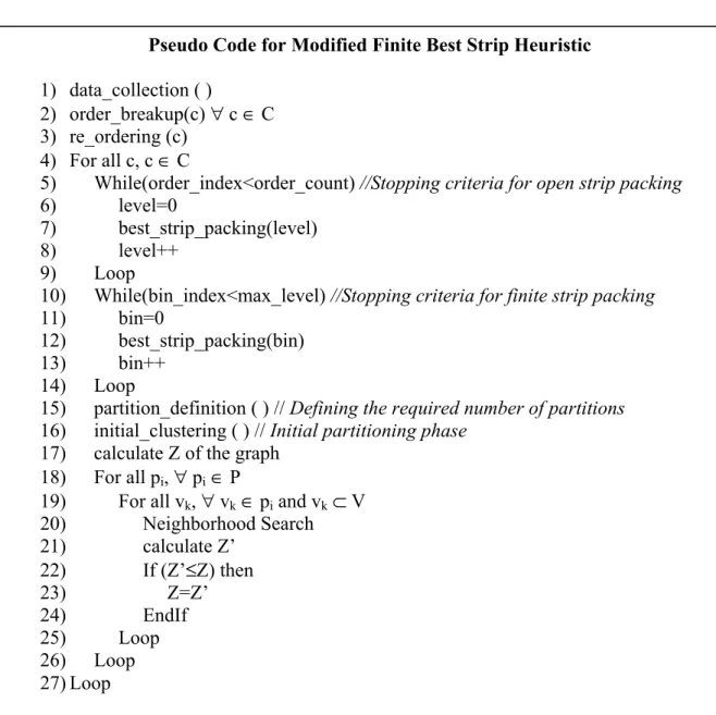
3.5 Pseudo Code
A pseudo code for the modified finite best strip packing heuristic and regrouping using k-way graph partitioning approach is shown in Figure 6.
Initially (line-1) the function data_collection ( ) is used to obtain order information from the user. The order is broken up (line-2) to meet the machine loading capacities. Breaking up of the order is done separately for different colors ‘c’. ‘C’ is the set containing all the different colors. The broken orders based on colors (Line-3) are reordered in non-increasing order of length and then on non-non-increasing order of width.
We begin the best fit heuristic from line-4. Initially in line-6 the levels are initialized. The best-strip packing algorithm for open-ended strip is run for each level (Line-7). A diagrammatic of this procedure is shown in Figure 6. Then once the packing on a particular level is complete, next level is initialized (Line-8). This procedure is repeated till all the orders have been packed into the open strip.
The variable max_level determines the total number of levels been created. For the finite strip packing each of the levels created previously act as individual rectangular pieces with length defined by height of that level and width defined by width of the open strip. In Line-11 the bins are initialized. The same best-strip packing algorithm is run to place these pieces (levels) into finite bins (line-12). As the bins are filled and no more rectangular pieces could be packed, new bins are initialized to fill in the remaining pieces (Line-13).
To handle the problem of re-grouping using k-way graph partitioning approach, the initial number of required partitions are defined (Line-15). If # of bins < # of machines (which generally isn’t) then # of partitions = # of bins. It is presumed that the remaining machines will go idle. However if # of bins > # of machines, then # of partitions = # of
machines. Then based on the number of partitions created, initially all the bins are randomly distributed into each of the partitions (Line-16). However care is taken to have a uniform partition. This will become the initial solution for the graph. In Line-17 the
value for this graph is estimated based on the formula in equation 4. The neighborhood search is performed systematically for every partition (Line-18) and every node in the partition (Line-19). Here pi represents partition ‘i’, where pi ∈ P and ‘P’ is a set
containing a list of all partitions. In Line-19, vk represents vertex ‘k’, where all vk∈ pi and
vk ⊂ V. ‘V’ represents a set of all vertices in the graph and ‘pi’ represents a set of all the
vertices in partition ‘i’. The new value of the graph is computed (Line-21) and if new value Z’ ≤ Z, then the new solution replaces the previous best solution.
Pseudo Code for Modified Finite Best Strip Heuristic
1) data_collection ( )
2) order_breakup(c) ∀ c ∈ C 3) re_ordering (c)
4) For all c, c ∈ C
5) While(order_index<order_count) //Stopping criteria for open strip packing 6) level=0
7) best_strip_packing(level) 8) level++
9) Loop
10) While(bin_index<max_level) //Stopping criteria for finite strip packing 11) bin=0
12) best_strip_packing(bin) 13) bin++
14) Loop
15) partition_definition ( ) // Defining the required number of partitions 16) initial_clustering ( ) // Initial partitioning phase
17) calculate Z of the graph 18) For all pi, ∀ pi ∈ P
19) For all vk, ∀ vk ∈ pi and vk ⊂ V 20) Neighborhood Search 21) calculate Z’ 22) If (Z’≤Z) then 23) Z=Z’ 24) EndIf 25) Loop 26) Loop 27) Loop
4 Results and Observation
Here we present the results and observations on the packing efficiency of modified finite best-strip heuristic. We also see the effect of surplus estimation on the overall packing efficiency.
4.1 Computation setup
Since this program was developed keeping in mind the problem scenario at CCX Inc, to run the experiments datasets from their monthly production run were considered. The measurement standards, conventions and other parameters like bin-size, machine capacity etc., are as per CCX Inc. Datasets of various sizes were considered to observe the performance of the algorithm.
4.2 Performance of modified finite best-strip heuristic
The experiments were run on a Pentium III- 800 processor. During the experimentation it was observed that the algorithm performs better with higher number pieces.
4.2.1 Packing Efficiency
The best-case performance was observed in all the cases was 98.18%. All bins have a default machine allowance of 1” on each side all along the length. Thus effectively we would have a minimum scrap of 1” on each side. For a bin of size 15,000” X 110”, the minimum scrap would be 15,000” X 2”. The efficiency drop from 100% to 98.18% is attributed to this effect. The worst-case performance was observed in dataset-5 with 30.91%. Also with the increase in # of pieces we observe an improvement in the average # of pieces packed per bin.
4.2.2 Upper bound
There has been several worst case upper bounds proposed for the two-dimensional open-ended bin-packing problem. The best-known upper bound for a finite-bin packing is by the hybrid first-fit algorithm which is given by N = 2.125 N* + 5. However here we observe a better performance by modified best-fit heuristic. The worst-case scenario has a performance given by N = 1.31 N*.
The performance of best fit heuristic as described in Berkey et. al [3] observes the yield
ratio of 1.04 . # . # ≈ reqd bins of Min packed bins of Actual
. We obtained the yield ratio slightly higher than the best fit heuristic. This is mainly attributed to the addition of guillotine cutting constraints. Dataset # (a) # of pieces (b) Avg. # of pieces per bin
(c)
Min. # of bins reqd. [N*]
(d)
Largest bin size Lx W [inches] (e) # of bins used (f) η 9 (g) Yield Ratio (h) = f/d Computation Time10 [Secs] (i) 1 236 2.12 84.35 15,000 X 110 111 76.25% 1.31 9.74 2 342 2.65 114.05 15,000 X 110 128 88.84% 1.12 13.28 3 668 2.19 266.86 15,000 X 110 303 88.02% 1.13 33.85 4 1153 2.62 405.80 15,000 X 110 439 91.90% 1.08 68.36 5 1460 2.80 486.15 15,000 X 110 518 92.84% 1.07 81.79 6 2279 2.84 746.42 15,000 X 110 799 91.19% 1.07 220.58 7 2810 2.78 922.17 15,000 X 110 1010 91.83% 1.09 383.33
Table 1: Summary of results for Modified Finite Best-Fit Heuristic
9
Average Efficiency of space utilization
10
4.3 Performance of k-way graph partitioning algorithm
The key factors, which affect the speed and performance of the k-way graph-partitioning algorithm, are:
1) Size of the graph
2) # of partitions
3) Degree of imbalance allowed (α).
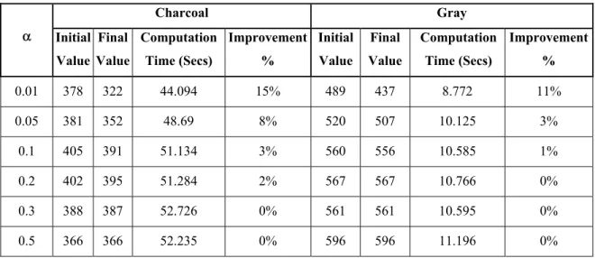
The number of bins generated by modified best-fit heuristic determines the size of the graph. The number of machines available determines the number of partitions in the graph. The degree of imbalance allowed (α) largely affects the performance, which is clearly indicated in Table 2. These trials were conducted for dataset-4. The graph consisted on 1153 vertices and 52 partitions. We can observe that for low values of α we obtain higher improvement in the solution and also reduction in computation time. But with lower values of α is associated higher imbalance in the graph which is also undesirable. Hence we have to come up with a compromising value. As from Table 2 we can observe that α value of 0.1 is quite reasonable.
Charcoal Gray α Initial Value Final Value Computation Time (Secs) Improvement % Initial Value Final Value Computation Time (Secs) Improvement % 0.01 378 322 44.094 15% 489 437 8.772 11% 0.05 381 352 48.69 8% 520 507 10.125 3% 0.1 405 391 51.134 3% 560 556 10.585 1% 0.2 402 395 51.284 2% 567 567 10.766 0% 0.3 388 387 52.726 0% 561 561 10.595 0% 0.5 366 366 52.235 0% 596 596 11.196 0%
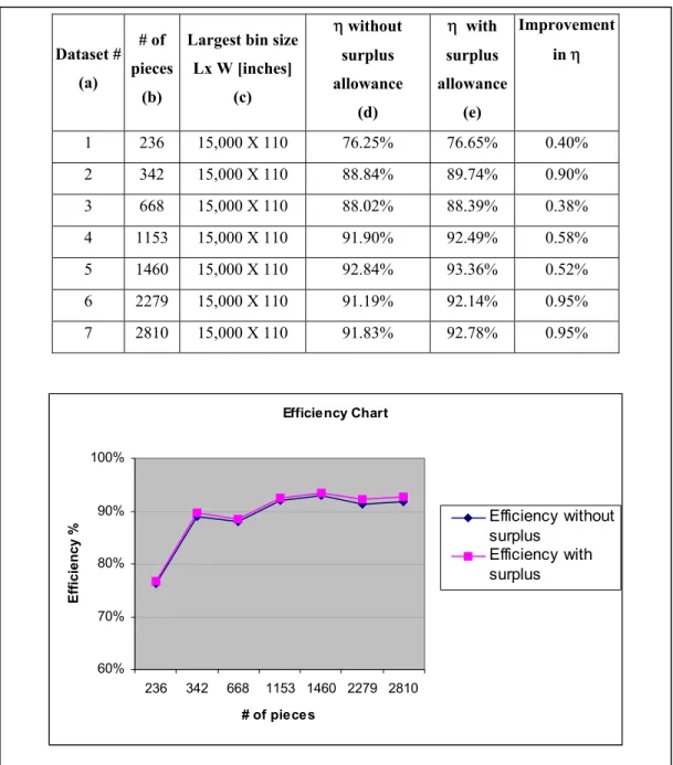
4.4 Effect of Surplus estimation
The estimation of surplus quantity was initially thought to make significant improvement to the obtained solution. However it appears that the degree of effect of surplus allowance doesn’t improve the obtained solution significantly. This could be attributed to the efficiency of the modified best-fit heuristic algorithm. The effect of surplus allowance is shown in Figure 7 Dataset # (a) # of pieces (b)
Largest bin size Lx W [inches] (c) η without surplus allowance (d) η with surplus allowance (e) Improvement in η 1 236 15,000 X 110 76.25% 76.65% 0.40% 2 342 15,000 X 110 88.84% 89.74% 0.90% 3 668 15,000 X 110 88.02% 88.39% 0.38% 4 1153 15,000 X 110 91.90% 92.49% 0.58% 5 1460 15,000 X 110 92.84% 93.36% 0.52% 6 2279 15,000 X 110 91.19% 92.14% 0.95% 7 2810 15,000 X 110 91.83% 92.78% 0.95% Efficiency Chart 60% 70% 80% 90% 100% 236 342 668 1153 1460 2279 2810 # of pieces Effi ci ency % Efficiency without surplus Efficiency with surplus
4.5 Concluding remarks
To measure the performance of modified finite best-fit heuristic various datasets were considered. The datasets were excerpts from the monthly production plan of CCX Technologies. The algorithm performed better on larger datasets. The best-case performance was 98.18% and the worst-case performance of 30.91%. There was an improvement in the upper bound from the previously best-known upper bound. The effect of surplus allowance was not significant.
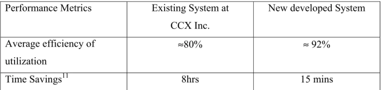
Benefits of this system:
Performance Metrics Existing System at
CCX Inc.
New developed System
Average efficiency of utilization
≈80% ≈ 92%
Time Savings11 8hrs 15 mins
Table 3: Performance Analysis of Existing System Vs. New developed System
From Table 3 we can observe a cost benefit in terms of both material value and time.
11
5 Summary and future scope of work
A problem of cost minimization due to material wastages as proposed by CCX Inc was considered. The problem was analyzed and determined to be finite-2-Dimensional Bin Backing problem with guillotine constraints. A general case of finite best-strip heuristic with no guillotine constraints was considered and modified suitably to include guillotine constraints. This modified best-strip heuristic’s performance when compared with general best-strip heuristic without any guillotine constraints was quite good. Also during implementation the issue of order tracking was encountered. This was quite successfully solved using k-way graph partitioning approach.
There is quite a bit of scope for further usage and improvement on this technique for solving problems of similar kind. There are 3 main categories for further research: Additional experimentation, enhancing the heuristic and
Additional Experimentation: This problem was solved only for a few datasets as provided by the company. The performance analysis for very large datasets can be explored.
Enhancing the heuristic: Alternative heuristics such as Hybrid First-Fit heuristic and Finite Next-Fit heuristic could be implemented to solve this problem and thus compare the performance. An additional dimension to this problem that could be added is time. This would help this tool to also be used for scheduling. Also here each order has the same priority. But it could happen some times that a particular order has higher priority than another one. This happens primarily when some orders are made to ship and some are made to stock. So a value could be associated with each order. This acts as an additional variable for optimization.
Interface with ERP module: This tool can be incorporated into the scheduling module of the ERP system. The master production schedule when generated by the planning department can be fed as an input into this tool and the system would come up with machine loading and cutting sequence, which would enable cost savings in terms of
a) Material costs (wastage minimization).
b) Setup costs (Machine loading sequence).
6 References
1. S Martello and D Vigo “Exact Solution of the Two-Dimensional Finite Bin
Packing Problem”, Management Science, Vol. 44, No. 3. (Mar., 1998), pp. 388-399.
2. N Christofides and C Whitlock “An Algorithm for two-Dimensional Cutting
Problems”, Operations Research, Vol. 25, No. 1. (Feb., 1977), pp. 30-44.
3. J.O. Berkey and P.Y. Wang “Two-Dimensional Finite Bin-Packing Algorithms”,
The Journal of Operational Research Society, Vol. 38, No. 5. (May., 1987), pp.
423-429.
4. B. Chazelle “The bottom-left bin-packing heuristic: an efficient implementation”
7 Appendix – I
Screenshots and images of the tool developed for CCX Technologies.
1. Data Input
Figure 8: Screen image of Input Form
Figure 8 represents the screen image for user input. The input parameters are Order #, Width, Length, Due Date and Color, which is entered in the spreadsheet provided. A check box for surplus calculation option is provided. Upon clicking the Calculate button, the program is executed.
2. Output Form
Figure 9: Screen image of Input Form
The program after execution display’s the output form. Figure 9 shows the screen image for the output form.
Upon selection of the Color, Loom # (Machine #) and Batch #, the allocation is
displayed in the following format.
Width X Length (Order#) E.g.: 28 X 15000 (41)
The utilization factor for the selected batch is displayed.
100 (%)= × TotalArea UsedArea nFactor Utilizatio
To get a summary report click on View Report. The summary report can be
printed on to any printer setup on the PC or can be exported as a file in html/text format.