Proceedings of the 56th Annual Meeting of the Association for Computational Linguistics (Long Papers), pages 317–327 317
Sentence-State LSTM for Text Representation
Yue Zhang1, Qi Liu1 and Linfeng Song2 1Singapore University of Technology and Design
2Department of Computer Science, University of Rochester
{yue zhang, qi liu}@sutd.edu.sg, lsong10@cs.rochester.edu
Abstract
Bi-directional LSTMs are a powerful tool for text representation. On the other hand, they have been shown to suffer var-ious limitations due to their sequential na-ture. We investigate an alternative LSTM structure for encoding text, which consists of a parallel state for each word. Re-current steps are used to perform local and global information exchange between words simultaneously, rather than incre-mental reading of a sequence of words. Results on various classification and se-quence labelling benchmarks show that the proposed model has strong representa-tion power, giving highly competitive per-formances compared to stacked BiLSTM models with similar parameter numbers.
1 Introduction
Neural models have become the dominant ap-proach in the NLP literature. Compared to hand-crafted indicator features, neural sentence repre-sentations are less sparse, and more flexible in en-coding intricate syntactic and semantic informa-tion. Among various neural networks for encod-ing sentences, bi-directional LSTMs (BiLSTM) (Hochreiter and Schmidhuber, 1997) have been a dominant method, giving state-of-the-art results in language modelling (Sundermeyer et al., 2012), machine translation (Bahdanau et al.,2015), syn-tactic parsing (Dozat and Manning, 2017) and question answering (Tan et al.,2015).
Despite their success, BiLSTMs have been shown to suffer several limitations. For example, their inherently sequential nature endows com-putation non-parallel within the same sentence (Vaswani et al.,2017), which can lead to a compu-tational bottleneck, hindering their use in the
in-...
...
...
...
...
...
...
...
time
0 1
...
t-1
[image:1.595.316.517.221.378.2]t
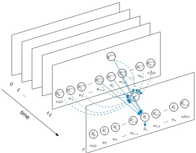
Figure 1: Sentence-State LSTM
dustry. In addition, local ngrams, which have been shown a highly useful source of contextual infor-mation for NLP, are not explicitly modelled (Wang et al.,2016). Finally, sequential information flow leads to relatively weaker power in capturing long-range dependencies, which results in lower perfor-mance in encoding longer sentences (Koehn and Knowles,2017).
At each recurrent step, information exchange is conducted between consecutive words in the sen-tence, and between the sentence-level state and each word. In particular, each word receives in-formation from its predecessor and successor si-multaneously. From an initial state without infor-mation exchange, each word-level state can obtain 3-gram, 5-gram and 7-gram information after 1, 2 and 3 recurrent steps, respectively. Being con-nected with every word, the sentence-level state vector serves to exchange non-local information with each word. In addition, it can also be used as a global sentence-level representation for clas-sification tasks.
Results on both classification and sequence la-belling show that S-LSTM gives better accuracies compared to BiLSTM using the same number of parameters, while being faster. We release our code and models at https://github.com/ leuchine/S-LSTM, which include all base-lines and the final model.
2 Related Work
LSTM (Graves and Schmidhuber, 2005) showed its early potentials in NLP when a neural machine translation system that leverages LSTM source encoding gave highly competitive results com-pared to the best SMT models (Bahdanau et al.,
2015). LSTM encoders have since been explored for other tasks, including syntactic parsing (Dyer et al.,2015), text classification (Yang et al.,2016) and machine reading (Hermann et al.,2015). Bi-directional extensions have become a standard configuration for achieving state-of-the-art accu-racies among various tasks (Wen et al.,2015;Ma and Hovy, 2016;Dozat and Manning, 2017). S-LSTMs are similar to BiS-LSTMs in their recurrent bi-directional message flow between words, but different in the design of state transition.
CNNs (Krizhevsky et al.,2012) also allow bet-ter parallelisation compared to LSTMs for sen-tence encoding (Kim,2014), thanks to parallelism among convolution filters. On the other hand, covolution features embody only fix-sized local n-gram information, whereas sentence-level feature aggregation via pooling can lead to loss of infor-mation (Sabour et al.,2017). In contrast, S-LSTM uses a global sentence-level node to assemble and back-distribute local information in the recurrent state transition process, suffering less information loss compared to pooling.
Attention (Bahdanau et al.,2015) has recently been explored as a standalone method for sentence encoding, giving competitive results compared to Bi-LSTM encoders for neural machine translation (Vaswani et al.,2017). The attention mechanism allows parallelisation, and can play a similar role to the sentence-level state in S-LSTMs, which uses neural gates to integrate word-level information compared to hierarchical attention. S-LSTM fur-ther allows local communication between neigh-bouring words.
Hierarchical stacking of CNN layers (LeCun et al., 1995; Kalchbrenner et al., 2014; Papan-dreou et al., 2015; Dauphin et al., 2017) allows better interaction between non-local components in a sentence via incremental levels of abstraction. S-LSTM is similar to hierarchical attention and stacked CNN in this respect, incrementally refin-ing sentence representations. However, S-LSTM models hierarchical encoding of sentence structure as a recurrentstate transition process. In nature, our work belongs to the family of LSTM sentence representations.
S-LSTM is inspired by message passing over graphs (Murphy et al.,1999;Scarselli et al.,2009). Graph-structure neural models have been used for computer program verification (Li et al.,2016) and image object detection (Liang et al., 2016). The closest previous work in NLP includes the use of convolutional neural networks (Bastings et al.,
2017; Marcheggiani and Titov, 2017) and DAG LSTMs (Peng et al.,2017) for modelling syntactic structures. Compared to our work, their motiva-tions and network structures are highly different. In particular, the DAG LSTM ofPeng et al.(2017) is a natural extension of tree LSTM (Tai et al.,
2015), and is sequential rather than parallel in na-ture. To our knowledge, we are the first to investi-gate a graph RNN for encoding sentences, propos-ing parallel graph states for integratpropos-ing word-level and sentence-level information. In this perspec-tive, our contribution is similar to that of Kim
(2014) andBahdanau et al.(2015) in introducing a neural representation to the NLP literature.
3 Model
Given a sentence s = w1, w2, . . . , wn, where wi represents the ith word and n is the sentence
length, our goal is to find a neural representation ofs, which consists of a hidden vectorhifor each
hid-den vectorg. Herehi represents syntactic and
se-mantic features forwiunder the sentential context,
whilegrepresents features for the whole sentence. Following previous work, we additionally addhsi
andh/sito the two ends of the sentence asw0and wn+1, respectively.
3.1 Baseline BiLSTM
The baseline BiLSTM model consists of two LSTM components, which process the input in the forward left-to-right and the backward right-to-left directions, respectively. In each direction, the reading of input words is modelled as a recur-rent process with a single hidden state. Given an initial value, the state changes its value recurrently, each time consuming an incoming word.
Take the forward LSTM component for exam-ple. Denoting the initial state as →h0, which is a model parameter, the recurrent state transition step for calculating→h1, . . . ,→hn+1 is defined as follows (Graves and Schmidhuber,2005):
ˆit=σ(W
ixt+Ui
→
ht−1+bi)
ˆ
ft=σ(Wfxt+Uf
→
ht−1+bf)
ot =σ(Woxt+Uo
→
ht−1+bo)
ut =tanh(Wuxt+Uu
→
ht−1+bu)
it,ft=softmax(ˆit,fˆt)
ct=ct−1ft+utit →
ht=ottanh(ct)
(1)
where xt denotes the word representation ofwt;
it,ot, ftandut represent the values of an input gate, an output gate, a forget gate and an actual in-put at time stept, respectively, which controls the information flow for a recurrent cell→ct and the state vector→ht;Wx,Uxandbx(x∈ {i, o, f, u})
are model parameters.σis the sigmoid function. The backward LSTM component follows the same recurrent state transition process as de-scribed in Eq1. Starting from an initial statehn+1, which is a model parameter, it reads the inputxn,
xn−1,. . .,x0, changing its value to
←
hn,←hn−1,
. . .,←h0, respectively. A separate set of parame-tersWˆx,Uˆxandˆbx(x∈ {i, o, f, u}) are used for
the backward component.
The BiLSTM model uses the concatenated value of→htand←htas the hidden vector forwt:
ht= [→ht;←ht]
A single hidden vector representation g of the whole input sentence can be obtained using the fi-nal state values of the two LSTM components:
g= [→hn+1;←h0]
Stacked BiLSTM Multiple layers of BiLTMs
can be stacked for increased representation power, where the hidden vectors of a lower layer are used as inputs for an upper layer. Different model pa-rameters are used in each stacked BiLSTM layer.
3.2 Sentence-State LSTM
Formally, an S-LSTM state at time stept can be denoted by:
Ht=hht0,h1t, . . . ,htn+1,gti,
which consists of a sub stateht
i for each wordwi
and a sentence-level sub stategt.
S-LSTM uses a recurrent state transition pro-cess to model information exchange between sub states, which enriches state representations incre-mentally. For the initial state H0, we set h0i =
g0 = h0, where h0 is a parameter. The state transition fromHt−1 toHt consists of sub state transitions from hti−1 tohit and fromgt−1 togt. We take an LSTM structure similar to the baseline BiLSTM for modelling state transition, using a re-current cellcti for eachwiand a cellctg forg.
As shown in Figure 1, the value of eachhti is computed based on the values ofxi, hti−−11, h
t−1 i ,
hti+1−1 andgt−1, together with their corresponding cell values:
ξit= [hti−−11,hti−1,hti+1−1] ˆit
i =σ(Wiξit+Uixi+Vigt−1+bi)
ˆ
lti =σ(Wlξti+Ulxi+Vlgt−1+bl)
ˆ
rit=σ(Wrξit+Urxi+Vrgt−1+br)
ˆ
fit=σ(Wfξit+Ufxi+Vfgt−1+bf)
ˆ
sti =σ(Wsξti+Usxi+Vsgt−1+bs)
oti =σ(Woξit+Uoxi+Vogt−1+bo)
uti =tanh(Wuξit+Uuxi+Vugt−1+bu)
iti,lti,rit,fit,sti =softmax(ˆiti,ˆlti,rˆit,fˆit,sˆti)
cti =lticit−−11+fitcti−1+ritcti+1−1
+sticgt−1+itiuti
hti =oittanh(cti)
(2)
gates that control information flow fromξitandxi
tocti. In particular, iti controls information from the inputxi;lti,rit,fitandsti control information
from the left context cell cti−−11, the right context cellcti+1−1,cit−1and the sentence context cellct−1
g ,
respectively. The values ofiti,lti,rit,fitandstiare normalised such that they sum to1. oti is an out-put gate from the cell statect
i to the hidden state
hti. Wx, Ux, Vx andbx (x ∈ {i, o, l, r, f, s, u})
are model parameters.σis the sigmoid function. The value ofgtis computed based on the values ofhti−1for alli∈[0..n+ 1]:
¯
h=avg(ht0−1,h1t−1, . . . ,htn+1−1) ˆ
fgt=σ(Wggt−1+Ug¯h+bg)
ˆ
fit=σ(Wfgt−1+Ufhti−1+bf)
ot=σ(Wogt−1+Uo¯h+bo)
f0t, . . . ,fn+1t ,fgt=softmax(fˆ0t, . . . ,fˆn+1t ,fˆgt)
ctg =fgtctg−1+X
i
fitcti−1
gt=ottanh(ctg)
(3) where ft
0, . . . ,fn+1t and fgt are gates controlling
information from ct0−1, . . . ,cn+1t−1 and ctg−1, re-spectively, which are normalised. otis an output gate from the recurrent cellctg togt.Wx,Uxand
bx(x∈ {g, f, o}) are model parameters.
Contrast with BiLSTM The difference
be-tween S-LSTM and BiLSTM can be understood with respect to their recurrent states. While BiL-STM uses only one state in each direction to rep-resent the subsequence from the beginning to a certain word, S-LSTM uses a structural state to represent the full sentence, which consists of a sentence-level sub state andn+ 2word-level sub states, simultaneously. Different from BiLSTMs, for whichhtat different time steps are used to rep-resentw0, . . . , wn+1, respectively, the word-level
stateshti and sentence-level stategtof S-LSTMs directly correspond to the goal outputs hi andg,
as introduced in the beginning of this section. As
t increases from 0, hti and gt are enriched with increasingly deeper context information.
From the perspective of information flow, BiL-STM passes information from one end of the sen-tence to the other. As a result, the number of time steps scales with the size of the input. In con-trast, S-LSTM allows bi-directional information flow at each word simultaneously, and additionally
between the sentence-level state and every word-level state. At each step, eachhi captures an
in-creasing larger ngram context, while additionally communicating globally to all otherhjviag. The
optimal number of recurrent steps is decided by the end-task performance, and does not necessar-ily scale with the sentence size. As a result, S-LSTM can potentially be both more efficient and more accurate compared with BiLSTMs.
Increasing window size. By default S-LSTM exchanges information only between neighbour-ing words, which can be seen as adoptneighbour-ing a 1-word window on each side. The window size can be extended to 2, 3 or more words in order to allow more communication in a state transi-tion, expediting information exchange. To this end, we modify Eq 2, integrating additional con-text words to ξti, with extended gates and cells. For example, with a window size of 2, ξti = [hti−−12,hti−−11,hti−1,hi+1t−1,hti+2−1]. We study the ef-fectiveness of window size in our experiments.
Additional sentence-level nodes. By default S-LSTM uses one sentence-level node. One way of enriching the parameter space is to add more sentence-level nodes, each communicating with word-level nodes in the same way as described by Eq 3. In addition, different sentence-level nodes can communicate with each other during state transition. When one sentence-level node is used for classification outputs, the other sentence-level node can serve as hidden memory units, or latent features. We study the effectiveness of mul-tiple sentence-level nodes empirically.
3.3 Task settings
We consider two task settings, namely classifica-tion and sequence labelling. Forclassification, g
is fed to asoftmaxclassification layer:
y=softmax(Wcg+bc)
where y is the probability distribution of output class labels andWcandbcare model parameters.
Forsequence labelling, eachhican be used as
fea-ture representation for a corresponding wordwi.
Dataset Training Development Test #sent #words #sent #words #sent #words
Movie review (Pang and Lee,2008) 8527 201137 1066 25026 1066 25260
Books 1400 297K 200 59K 400 68K
Electronics 1398 924K 200 184K 400 224K
DVD 1400 1,587K 200 317K 400 404K
Kitchen 1400 769K 200 153K 400 195K
Apparel 1400 525K 200 105K 400 128K
Camera 1397 1,084K 200 216K 400 260K
Text Health 1400 742K 200 148K 400 175K
Classification Music 1400 1,176K 200 235K 400 276K
(Liu et al.,2017) Toys 1400 792K 200 158K 400 196K
Video 1400 1,311K 200 262K 400 342K
Baby 1300 855K 200 171K 400 221K
Magazines 1370 1,033K 200 206K 400 264K
Software 1315 1,143K 200 228K 400 271K
Sports 1400 833K 200 183K 400 218K
IMDB 1400 2,205K 200 507K 400 475K
MR 1400 196K 200 41K 400 48K
POS tagging (Marcus et al.,1993) 39831 950011 1699 40068 2415 56671
[image:5.595.72.298.61.230.2]NER (Sang et al.,2003) 14987 204567 3466 51578 3684 46666
Table 1: Dataset statistics
et al.,2015) is applied to the hidden states of input words for both BiLSTMs and S-LSTMs calculat-ing a weighted sum
g=X
t αtht
where
αt=
expuT t
P
iexpuTi
t=tanh(Wαht+bα)
HereWα,uandbαare model parameters.
External CRF For sequential labelling, we use a CRF layer on top of the hidden vec-torsh1,h2, . . . ,hnfor calculating the conditional
probabilities of label sequences (Huang et al.,
2015;Ma and Hovy,2016):
P(Y1n|h,Ws,bs) =
Qn
i=1ψi(yi−1, yi,h)
P
Yn0
1
Qn
i=1ψi(y0i−1, yi0,h)
ψi(yi−1, yi,h) =exp(W yi−1,yi
s hi+b yi−1,yi
s )
where Wyi−1,yi
s and bysi−1,yi are parameters
spe-cific to two consecutive labelsyi−1andyi.
For training, standard log-likelihood loss is used withL2regularization given a set of gold-standard
instances.
4 Experiments
We empirically compare S-LSTMs and BiLSTMs on different classification and sequence labelling tasks. All experiments are conducted using a GeForce GTX 1080 GPU with 8GB memory.
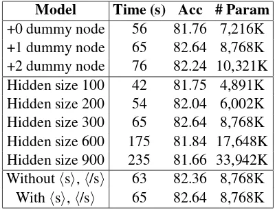
Model Time (s) Acc # Param
+0 dummy node 56 81.76 7,216K +1 dummy node 65 82.64 8,768K +2 dummy node 76 82.24 10,321K Hidden size 100 42 81.75 4,891K Hidden size 200 54 82.04 6,002K Hidden size 300 65 82.64 8,768K Hidden size 600 175 81.84 17,648K Hidden size 900 235 81.66 33,942K Withouthsi,h/si 63 82.36 8,768K
Withhsi,h/si 65 82.64 8,768K
Table 2: Movie review DEVresults of S-LSTM
4.1 Experimental Settings
Datasets. We choose the movie review dataset of Pang and Lee (2008), and additionally the 16 datasets ofLiu et al. (2017) for classification evaluation. We randomly split the movie review dataset into training (80%), development (10%) and test (10%) sections, and the original split of
Liu et al.(2017) for the 16 classification datasets. For sequence labelling, we choose the Penn Treebank (Marcus et al.,1993) POS tagging task and the CoNLL (Sang et al., 2003) NER task as our benchmarks. For POS tagging, we follow the standard split (Manning,2011), using sections 0 – 18 for training, 19 – 21 for development and 22 – 24 for test. For NER, we follow the standard split, and use the BIOES tagging scheme (Ratinov and Roth,2009). Statistics of the four datasets are shown in Table1.
Hyperparameters. We initialise word embed-dings using GloVe (Pennington et al., 2014) 300 dimensional embeddings.1 Embeddings are fine-tuned during model training for all tasks. Dropout (Srivastava et al., 2014) is applied to embedding hidden states, with a rate of 0.5. All models are optimised using the Adam optimizer (Kingma and Ba, 2014), with an initial learning rate of 0.001 and a decay rate of 0.97. Gradients are clipped at 3 and a batch size of 10 is adopted. Sentences with similar lengths are batched together. The L2 regularization parameter is set to 0.001.
4.2 Development Experiments
We use the movie review development data to in-vestigate different configurations of S-LSTMs and BiLSTMs. For S-LSTMs, the default configura-tion useshsiandh/siwords for augmenting words
[image:5.595.316.516.62.215.2]1
3
5
7
9
11
Time Step t
0.795
0.800
0.805
0.810
0.815
0.820
0.825
0.830
Accuracy
window = 1 [image:6.595.82.280.58.204.2]window = 2 window = 3 window = 4
Figure 2: Accuracies with various window sizes and time steps on movie review development set
of a sentence. A hidden layer size of 300 and one sentence-level node are used.
Hyperparameters: Table2shows the develop-ment results of various S-LSTM settings, where Time refers to training time per epoch. Without the sentence-level node, the accuracy of S-LSTM drops to 81.76%, demonstrating the necessity of global information exchange. Adding one addi-tional sentence-level node as described in Sec-tion 3.2does not lead to accuracy improvements, although the number of parameters and decoding time increase accordingly. As a result, we use only 1 sentence-level node for the remaining experi-ments. The accuracies of S-LSTM increases as the hidden layer size for each node increases from 100 to 300, but does not further increase when the size increases beyond 300. We fix the hidden size to 300 accordingly. Without usinghsiandh/si, the performance of S-LSTM drops from 82.64% to 82.36%, showing the effectiveness of having these additional nodes. Hyperparameters for BiLSTM models are also set according to the development data, which we omit here.
State transition. In Table2, the number of re-current state transition steps of S-LSTM is decided according to the best development performance. Figure2 draws the development accuracies of S-LSTMs with various window sizes against the number of recurrent steps. As can be seen from the figure, when the number of time steps increases from 1 to 11, the accuracies generally increase, before reaching a maximum value. This shows the effectiveness of recurrent information exchange in S-LSTM state transition.
On the other hand, no significant differences are observed on the peak accuracies given by different window sizes, although a larger window size (e.g.
Model Time (s) Acc # Param
LSTM 67 80.72 5,977K BiLSTM 106 81.73 7,059K 2 stacked BiLSTM 207 81.97 9,221K 3 stacked BiLSTM 310 81.53 11,383K 4 stacked BiLSTM 411 81.37 13,546K S-LSTM 65 82.64* 8,768K
[image:6.595.306.528.62.281.2]CNN 34 80.35 5,637K 2 stacked CNN 40 80.97 5,717K 3 stacked CNN 47 81.46 5,808K 4 stacked CNN 51 81.39 5,855K Transformer (N=6) 138 81.03 7,234K Transformer (N=8) 174 81.86 7,615K Transformer (N=10) 214 81.63 8,004K BiLSTM+Attention 126 82.37 7,419K S-LSTM+Attention 87 83.07* 8,858K
Table 3: Movie review development results
4) generally results in faster plateauing. This can be be explained by the intuition that information exchange between distant nodes can be achieved using more recurrent steps under a smaller win-dow size, as can be achieved using fewer steps un-der a larger window size. Consiun-dering efficiency, we choose a window size of 1 for the remaining experiments, setting the number of recurrent steps to 9 according to Figure2.
S-LSTM vs BiLSTM: As shown in Table
3, BiLSTM gives significantly better accuracies compared to uni-directional LSTM2, with the training time per epoch growing from 67 seconds to 106 seconds. Stacking 2 layers of BiLSTM gives further improvements to development re-sults, with a larger time of 207 seconds. 3 lay-ers of stacked BiLSTM does not further improve the results. In contrast, S-LSTM gives a develop-ment result of 82.64%, which is significantly bet-ter compared to 2-layer stacked BiLSTM, with a smaller number of model parameters and a shorter time of 65 seconds.
We additionally make comparisons with stacked CNNs and hierarchical attention (Vaswani et al., 2017), shown in Table 3 (the CNN and Transformer rows), whereN indicates the number of attention layers. CNN is the most efficient among all models compared, with the smallest model size. On the other hand, a 3-layer stacked CNN gives an accuracy of 81.46%, which is also
2p < 0.01using t-test. For the remaining of this paper,
Model Accuracy Train (s) Test (s) Socher et al.(2011) 77.70 – –
Socher et al.(2012) 79.00 – –
Kim(2014) 81.50 – –
Qian et al.(2016) 81.50 – –
BiLSTM 81.61 51 1.62
[image:7.595.75.290.60.214.2]2 stacked BiLSTM 81.94 98 3.18 3 stacked BiLSTM 81.71 137 4.67 3 stacked CNN 81.59 31 1.04 Transformer (N=8) 81.97 89 2.75 S-LSTM 82.45* 41 1.53
Table 4: Test set results on movie review dataset (* denotes significance in all tables).
the lowest compared with BiLSTM, hierarchical attention and S-LSTM. The best performance of hierarchical attention is between single-layer and two-layer BiLSTMs in terms of both accuracy and efficiency. S-LSTM gives significantly better accuracies compared with both CNN and hierarchical attention.
Influence of external attention mechanism. Table3additionally shows the results of BiLSTM and S-LSTM when external attention is used as described in Section 3.3. Attention leads to im-proved accuracies for both BiLSTM and S-LSTM in classification, with S-LSTM still outperform-ing BiLSTM significantly. The result suggests that external techniques such as attention can play or-thogonal roles compared with internal recurrent structures, therefore benefiting both BiLSTMs and S-LSTMs. Similar observations are found using external CRF layers for sequence labelling.
4.3 Final Results for Classification
The final results on the movie review and rich text classification datasets are shown in Tables 4 and
5, respectively. In addition to training time per epoch, test times are additionally reported. We use the best settings on the movie review development dataset for both S-LSTMs and BiLSTMs. The step number for S-LSTMs is set to 9.
As shown in Table 4, the final results on the movie review dataset are consistent with the devel-opment results, where S-LSTM outperforms BiL-STM significantly, with a faster speed. Observa-tions on CNN and hierarchical attention are con-sistent with the development results. S-LSTM also gives highly competitive results when compared with existing methods in the literature.
1
3
5
7
9 11
S-LSTM Time Step
91.5
92.0
92.5
93.0
93.5
94.0
94.5
95.0
F1
(a) CoNLL03
1
3
5
7
9 11
S-LSTM Time Step
96.8
96.9
97.0
97.1
97.2
97.3
97.4
97.5
97.6
Accuracy
(b) WSJ
Figure 3: Sequence labelling development results.
As shown in Table5, among the 16 datasets of
Liu et al. (2017), S-LSTM gives the best results on 12, compared with BiLSTM and 2 layered BiL-STM models. The average accuracy of S-LBiL-STM is 85.6%, significantly higher compared with 84.9% by 2-layer stacked BiLSTM. 3-layer stacked BiL-STM gives an average accuracy of 84.57%, which is lower compared to a 2-layer stacked BiLSTM, with a training time per epoch of 423.6 seconds. The relative speed advantage of S-LSTM over BiLSTM is larger on the 16 datasets as compared to the movie review test test. This is because the average length of inputs is larger on the 16 datasets (see Section4.5).
4.4 Final Results for Sequence Labelling
Dataset SLSTM Time (s) BiLSTM Time (s) 2 BiLSTM Time (s)
Camera 90.02* 50 (2.85) 87.05 115 (8.37) 88.07 221 (16.1) Video 86.75* 55 (3.95) 84.73 140 (12.59) 85.23 268 (25.86) Health 86.5 37 (2.17) 85.52 118 (6.38) 85.89 227 (11.16) Music 82.04* 52 (3.44) 78.74 185 (12.27) 80.45 268 (23.46) Kitchen 84.54* 40 (2.50) 82.22 118 (10.18) 83.77 225 (19.77)
DVD 85.52* 63 (5.29) 83.71 166 (15.42) 84.77 217 (28.31)
Toys 85.25 39 (2.42) 85.72 119 (7.58) 85.82 231 (14.83)
Baby 86.25* 40 (2.63) 84.51 125 (8.50) 85.45 238 (17.73)
Books 83.44* 64 (3.64) 82.12 240 (13.59) 82.77 458 (28.82)
IMDB 87.15* 67 (3.69) 86.02 248 (13.33) 86.55 486 (26.22)
MR 76.2 27 (1.25) 75.73 39 (2.27) 75.98 72 (4.63) Appeal 85.75 35 (2.83) 86.05 119 (11.98) 86.35* 229 (22.76) Magazines 93.75* 51 (2.93) 92.52 214 (11.06) 92.89 417 (22.77) Electronics 83.25* 47 (2.55) 82.51 195 (10.14) 82.33 356 (19.77) Sports 85.75* 44 (2.64) 84.04 172 (8.64) 84.78 328 (16.34) Software 87.75* 54 (2.98) 86.73 245 (12.38) 86.97 459 (24.68)
[image:8.595.79.519.62.310.2]Average 85.38* 47.30 (2.98) 84.01 153.48 (10.29) 84.64 282.24 (20.2)
Table 5: Results on the 16 datasets ofLiu et al.(2017). Time format: train (test)
Model Accuracy Train (s) Test (s)
Manning(2011) 97.28 – –
Collobert et al.(2011) 97.29 – –
Sun(2014) 97.36 – –
Søgaard(2011) 97.50 – –
Huang et al.(2015) 97.55 – –
Ma and Hovy(2016) 97.55 – –
Yang et al.(2017) 97.55 – –
BiLSTM 97.35 254 22.50
2 stacked BiLSTM 97.41 501 43.99 3 stacked BiLSTM 97.40 746 64.96
[image:8.595.73.293.347.515.2]S-LSTM 97.55 237 22.16
Table 6: Results on PTB (POS tagging)
the number of recurrent steps on the respective de-velopment sets for sequence labelling. The POS accuracies and NER F1-scores against the number of recurrent steps are shown in Figure 3 (a) and (b), respectively. For POS tagging, the best step number is set to 7, with a development accuracy of 97.58%. For NER, the step number is set to 9, with a development F1-score of 94.98%.
As can be seen in Table6, S-LSTM gives signif-icantly better results compared with BiLSTM on the WSJ dataset. It also gives competitive accu-racies as compared with existing methods in the literature. Stacking two layers of BiLSTMs leads to improved results compared to one-layer BiL-STM, but the accuracy does not further improve
Model F1 Train (s) Test (s)
Collobert et al.(2011) 89.59 – –
Passos et al.(2014) 90.90 – –
Luo et al.(2015) 91.20 – –
Huang et al.(2015) 90.10 – –
Lample et al.(2016) 90.94 – –
Ma and Hovy(2016) 91.21 – –
Yang et al.(2017) 91.26 – –
Rei(2017) 86.26 – –
Peters et al.(2017) 91.93 – –
BiLSTM 90.96 82 9.89
2 stacked BiLSTM 91.02 159 18.88 3 stacked BiLSTM 91.06 235 30.97 S-LSTM 91.57* 79 9.78
Table 7: Results on CoNLL03 (NER)
with three layers of stacked LSTMs.
For NER (Table7), S-LSTM gives an F1-score of 91.57% on the CoNLL test set, which is sig-nificantly better compared with BiLSTMs. Stack-ing more layers of BiLSTMs leads to slightly bet-ter F1-scores compared with a single-layer BiL-STM. Our BiLSTM results are comparable to the results reported byMa and Hovy(2016) and Lam-ple et al.(2016), who also use bidirectional RNN-CRF structures. In contrast, S-LSTM gives the best reported results under the same settings.
In the second section of Table 7, Yang et al.
10
20
30
40
50
60
Length
0.70
0.75
0.80
0.85
0.90
Accuracy
BiLSTM S-LSTM
(a) Movie review
20 40 60 80 100 120
Length
0.92
0.93
0.94
0.95
0.96
0.97
0.98
0.99
1.00
F1
BiLSTM S-LSTM
[image:9.595.87.275.59.396.2](b) CoNLL03
Figure 4: Accuracies against sentence length.
learning using additional language model objec-tives, obtaining an F-score of 86.26%;Peters et al.
(2017) leverage character-level language models, obtaining an F-score of 91.93%, which is the cur-rent best result on the dataset. All the three mod-els are based on BiLSTM-CRF. On the other hand, these semi-supervised learning techniques are or-thogonal to our work, and can potentially be used for S-LSTM also.
4.5 Analysis
Figure 4 (a) and (b) show the accuracies against the sentence length on the movie review and CoNLL datasets, respectively, where test samples are binned in batches of 80. We find that the per-formances of both S-LSTM and BiLSTM decrease as the sentence length increases. On the other hand, S-LSTM demonstrates relatively better ro-bustness compared to BiLSTMs. This confirms our intuition that a sentence-level node can facili-tate better non-local communication.
Figure 5 shows the training time per epoch of S-LSTM and BiLSTM on sentences with different lengths on the 16 classification datasets. To make
16.7 29.9 43.8 59.4 76.7 97.6 124.4161.6226.8484.3Avg Length
0 100 200 300 400 500 600
Time (s)
[image:9.595.322.504.62.185.2]BiLSTM S-LSTM
Figure 5: Time against sentence length.
these comparisons, we mix all training instances, order them by the size, and put them into 10 equal groups, the medium sentence lengths of which are shown. As can be seen from the figure, the speed advantage of S-LSTM is larger when the size of the input text increases, thanks to a fixed number of recurrent steps.
Similar to hierarchical attention (Vaswani et al.,
2017), there is a relative disadvantage of S-LSTM in comparison with BiLSTM, which is that the memory consumption is relatively larger. For ex-ample, over the movie review development set, the actual GPU memory consumption by S-LSTM, BiLSTM, 2-layer stacked BiLSTM and 4-layer stacked BiLSTM are 252M, 89M, 146M and 253M, respectively. This is due to the fact that computation is performed in parallel by S-LSTM and hierarchical attention.
5 Conclusion
We have investigated S-LSTM, a recurrent neu-ral network for encoding sentences, which offers richer contextual information exchange with more parallelism compared to BiLSTMs. Results on a range of classification and sequence labelling tasks show that S-LSTM outperforms BiLSTMs using the same number of parameters, demonstrat-ing that S-LSTM can be a useful addition to the neural toolbox for encoding sentences.
The structural nature in S-LSTM states allows straightforward extension to tree structures, result-ing in highly parallelisable tree LSTMs. We leave such investigation to future work. Next directions also include the investigation of S-LSTM to more NLP tasks, such as machine translation.
Acknowledge
References
Dzmitry Bahdanau, Kyunghyun Cho, and Yoshua Ben-gio. 2015. Neural machine translation by jointly learning to align and translate. InICLR 2015.
Joost Bastings, Ivan Titov, Wilker Aziz, Diego Marcheggiani, and Khalil Simaan. 2017. Graph convolutional encoders for syntax-aware neural ma-chine translation. InProceedings of EMNLP 2017. Copenhagen, Denmark, pages 1957–1967.
Ronan Collobert, Jason Weston, L´eon Bottou, Michael Karlen, Koray Kavukcuoglu, and Pavel Kuksa. 2011. Natural language processing (almost) from scratch. JMLR12(Aug):2493–2537.
Yann N Dauphin, Angela Fan, Michael Auli, and David Grangier. 2017. Language modeling with gated con-volutional networks. InICML. pages 933–941.
Timothy Dozat and Christopher D Manning. 2017. Deep biaffine attention for neural dependency pars-ing. InICLR 2017.
Chris Dyer, Miguel Ballesteros, Wang Ling, Austin Matthews, and Noah A. Smith. 2015. Transition-based dependency parsing with stack long short-term memory. InProceedings of ACL 2015. Beijing, China, pages 334–343.
Alex Graves and J¨urgen Schmidhuber. 2005. Frame-wise phoneme classification with bidirectional lstm and other neural network architectures. Neural Net-workspages 602–610.
Karl Moritz Hermann, Tomas Kocisky, Edward Grefenstette, Lasse Espeholt, Will Kay, Mustafa Su-leyman, and Phil Blunsom. 2015. Teaching ma-chines to read and comprehend. In NIPS. pages 1693–1701.
Sepp Hochreiter and J¨urgen Schmidhuber. 1997. Long short-term memory. Neural computation
9(8):1735–1780.
Zhiheng Huang, Wei Xu, and Kai Yu. 2015. Bidirec-tional lstm-crf models for sequence tagging. arXiv preprint arXiv:1508.01991.
Nal Kalchbrenner, Edward Grefenstette, and Phil Blun-som. 2014. A convolutional neural network for modelling sentences. InProceedings of ACL 2014. Baltimore, Maryland, pages 655–665.
Yoon Kim. 2014. Convolutional neural networks for sentence classification. InProceedings of EMNLP 2014. Doha, Qatar, pages 1746–1751.
Diederik P Kingma and Jimmy Ba. 2014. Adam: A method for stochastic optimization. arXiv preprint arXiv:1412.6980.
Philipp Koehn and Rebecca Knowles. 2017. Six chal-lenges for neural machine translation. In Pro-ceedings of the First Workshop on Neural Machine Translation. Vancouver, pages 28–39.
Alex Krizhevsky, Ilya Sutskever, and Geoffrey E Hin-ton. 2012. Imagenet classification with deep con-volutional neural networks. InNIPS. pages 1097– 1105.
Guillaume Lample, Miguel Ballesteros, Sandeep Sub-ramanian, Kazuya Kawakami, and Chris Dyer. 2016. Neural architectures for named entity recognition. InProceedings of the 2016 NAACL. San Diego, Cal-ifornia, pages 260–270.
Yann LeCun, Yoshua Bengio, et al. 1995. Convolu-tional networks for images, speech, and time series.
The handbook of brain theory and neural networks
3361(10):1995.
Yujia Li, Daniel Tarlow, Marc Brockschmidt, and Richard Zemel. 2016. Gated graph sequence neu-ral networks. InICLR 2016.
Xiaodan Liang, Xiaohui Shen, Jiashi Feng, Liang Lin, and Shuicheng Yan. 2016. Semantic object parsing with graph lstm. In ECCV. Springer, pages 125– 143.
Pengfei Liu, Xipeng Qiu, and Xuanjing Huang. 2017. Adversarial multi-task learning for text classifica-tion. In Proceedings of ACL 2017. Vancouver, Canada, pages 1–10.
Gang Luo, Xiaojiang Huang, Chin-Yew Lin, and Za-iqing Nie. 2015. Joint entity recognition and disam-biguation. InProceedings of EMNLP 2015. pages 879–888.
Xuezhe Ma and Eduard Hovy. 2016. End-to-end sequence labeling via bi-directional LSTM-CNNs-CRF. In Proceedings of ACL 2016. Berlin, Ger-many, pages 1064–1074.
Christopher D Manning. 2011. Part-of-speech tagging from 97% to 100%: is it time for some linguistics? InCICLing. Springer, pages 171–189.
Diego Marcheggiani and Ivan Titov. 2017. Encoding sentences with graph convolutional networks for se-mantic role labeling. In Proceedings of EMNLP 2017. Copenhagen, Denmark, pages 1506–1515.
Mitchell P Marcus, Mary Ann Marcinkiewicz, and Beatrice Santorini. 1993. Building a large annotated corpus of english: The penn treebank. Computa-tional linguistics19(2):313–330.
Kevin P Murphy, Yair Weiss, and Michael I Jordan. 1999. Loopy belief propagation for approximate in-ference: An empirical study. InUAI. Morgan Kauf-mann Publishers Inc., pages 467–475.
Bo Pang and Lillian Lee. 2008. Opinion mining and sentiment analysis. Foundations and TrendsR in In-formation Retrieval2(1–2):1–135.
Alexandre Passos, Vineet Kumar, and Andrew McCal-lum. 2014. Lexicon infused phrase embeddings for named entity resolution. In CoNLL. Ann Arbor, Michigan, pages 78–86.
Nanyun Peng, Hoifung Poon, Chris Quirk, Kristina Toutanova, and Wen-tau Yih. 2017. Cross-sentence n-ary relation extraction with graph lstms. Transac-tions of the Association for Computational Linguis-tics5:101–115.
Jeffrey Pennington, Richard Socher, and Christopher Manning. 2014. Glove: Global vectors for word representation. In Proceedings of EMNLP 2014. pages 1532–1543.
Matthew Peters, Waleed Ammar, Chandra Bhagavat-ula, and Russell Power. 2017. Semi-supervised se-quence tagging with bidirectional language models. In Proceedings of ACL 2017. Vancouver, Canada, pages 1756–1765.
Qiao Qian, Minlie Huang, Jinhao Lei, and Xi-aoyan Zhu. 2016. Linguistically regularized lstms for sentiment classification. arXiv preprint arXiv:1611.03949.
Lev Ratinov and Dan Roth. 2009. Design challenges and misconceptions in named entity recognition. In
CoNLL. pages 147–155.
Marek Rei. 2017. Semi-supervised multitask learning for sequence labeling. InProceedings of ACL 2017. Vancouver, Canada, pages 2121–2130.
Sara Sabour, Nicholas Frosst, and Geoffrey E Hinton. 2017. Dynamic routing between capsules. InNIPS. pages 3859–3869.
Tjong Kim Sang, Erik F, and De Meulder Fien. 2003. Introduction to the conll-2003 shared task: Language-independent named entity recognition. In
Proceedings of HLT-NAACL 2003-Volume 4. pages 142–147.
Franco Scarselli, Marco Gori, Ah Chung Tsoi, Markus Hagenbuchner, and Gabriele Monfardini. 2009. The graph neural network model. IEEE Transactions on Neural Networks20(1):61–80.
Richard Socher, Brody Huval, Christopher D Manning, and Andrew Y Ng. 2012. Semantic compositional-ity through recursive matrix-vector spaces. In Pro-ceedings of EMNLP 2012. pages 1201–1211.
Richard Socher, Jeffrey Pennington, Eric H Huang, Andrew Y Ng, and Christopher D Manning. 2011. Semi-supervised recursive autoencoders for predict-ing sentiment distributions. In Proceedings of EMNLP 2011. pages 151–161.
Anders Søgaard. 2011. Semisupervised condensed nearest neighbor for part-of-speech tagging. In Pro-ceedings of ACL 2011. pages 48–52.
Nitish Srivastava, Geoffrey Hinton, Alex Krizhevsky, Ilya Sutskever, and Ruslan Salakhutdinov. 2014. Dropout: A simple way to prevent neural networks from overfitting. JMLR15(1):1929–1958.
Xu Sun. 2014. Structure regularization for structured prediction. InNIPS. pages 2402–2410.
Martin Sundermeyer, Ralf Schl¨uter, and Hermann Ney. 2012. Lstm neural networks for language modeling. InInterSpeech.
Kai Sheng Tai, Richard Socher, and Christopher D. Manning. 2015. Improved semantic representations from tree-structured long short-term memory net-works. InProceedings of ACL 2015. Beijing, China, pages 1556–1566.
Ming Tan, Cicero dos Santos, Bing Xiang, and Bowen Zhou. 2015. Lstm-based deep learning models for non-factoid answer selection. arXiv preprint arXiv:1511.04108.
Ashish Vaswani, Noam Shazeer, Niki Parmar, Jakob Uszkoreit, Llion Jones, Aidan N Gomez, Łukasz Kaiser, and Illia Polosukhin. 2017. Attention is all you need. InNIPS. pages 6000–6010.
Xingyou Wang, Weijie Jiang, and Zhiyong Luo. 2016. Combination of convolutional and recurrent neural network for sentiment analysis of short texts. In
Proceedings of COLING 2016. pages 2428–2437.
Tsung-Hsien Wen, Milica Gasic, Nikola Mrkˇsi´c, Pei-Hao Su, David Vandyke, and Steve Young. 2015. Semantically conditioned lstm-based natural lan-guage generation for spoken dialogue systems. In
Proceedings of EMNLP 2015. Lisbon, Portugal, pages 1711–1721.
Zhilin Yang, Ruslan Salakhutdinov, and William W Cohen. 2017. Transfer learning for sequence tag-ging with hierarchical recurrent networks. InICLR 2017.
Zichao Yang, Diyi Yang, Chris Dyer, Xiaodong He, Alex Smola, and Eduard Hovy. 2016. Hierarchical attention networks for document classification. In