Munich Personal RePEc Archive
Dynamic Bunching Estimation with
Panel Data
Marx, Benjamin M.
University of Illinois at Urbana-Champaign
23 August 2018
Online at
https://mpra.ub.uni-muenchen.de/88647/
Dynamic Bunching Estimation with Panel Data
Benjamin M. Marx*
August 2018
Abstract
An increasingly common technique for studying behavioral elasticities uses bunching estimation of the excess mass in a distribution around a price or policy threshold. This paper shows how serial dependence of the choice variable and extensive-margin responses may bias these estimates. It then proposes new bunching designs that take greater advantage of panel data to avoid these biases and estimate new parameters. Standard methods over-reject in simulations using household income data and over-estimate bunching in an application with charities. Designs exploiting panel data provide unbiased bunching estimates, improved heterogeneity analysis, and the ability to estimate extensive-margin responses and long-run effects.
JEL: C23, D92, H21, H26.
1 Introduction
Taxes, income eligibility limits, and other policies can change agents’ incentives at threshold values of a choice variable. Some policies create a kink in the cost function at the threshold, while others create discontinuities, or “notches” (Slemrod, 2010). If costs increase above the threshold, the incentive to locate at or below the threshold can create “bunching” in the distribution of the choice variable. Saez (2010a) launched a bunching-estimation literature by showing how the extent of bunching around a kink in the tax schedule can be used to obtain an estimate of the tax price elasticity of income. The theory and technique of bunching estimation have been developed by Kleven and Waseem (2013), and bunching has been estimated at many kinks and notches in tax and regulatory schedules.1
This paper proposes and evaluates new “dynamic bunching estimation” designs for panel data. In the extant literature, researchers with access to panel datasets have treated them as repeated cross sections by pooling years. The methods proposed in this paper take greater advantage of the panel structure, and they offer improved identification and the ability to quantify parameters that have not been estimated with standard techniques. I examine two threats to identification for the standard design and show that the dynamic alternatives rely on assumptions that are arguably more plausible, particularly in settings where agents face a notch repeatedly. These designs can identify new parameters including long-run effects of a notch, which provide evidence on whether bunching is driven by retiming or misreporting, and the extent of extensive-margin responses to a notch. In addition, they offer new capabilities for analyzing heterogeneity in the bunching response and concurrent responses in other variables.
I first study two identification issues for the standard, static approach. One issue is extensive-margin responses, which have been discussed in the bunching literature but cannot be quantified with existing methods. Another issue that has not been discussed as an identification concern arises from persistent notches and serial dependence of the choice variable.2 To see the issue for identification, suppose there is a
tax notch that imposes a fixed cost when household income exceeds a threshold, and suppose that income exhibits positive serial dependence, i.e. that reducing income in the present will also reduce income in the future.3 When the notch is introduced, we would expect some households with potential incomes just above
1Recent papers estimating bunching have studied firms’ responses to taxes and regulations (Sallee and Slemrod 2012,
De-vereux et al. 2014, Best et al. 2015, Sallee and Ito 2018), individuals’ responses to taxes and benefits (Chetty et al. 2013a, Burman et al. 2014, Kleven and Schultz 2014, Kleven et al. 2014, Kline and Tartari 2016, Rees-Jones 2018), consumer responses to prices (Ito 2014, Grubb and Osborne 2015, Einav et al. 2017), saving (Ramnath 2013, Weber 2016), teacher responses to testing incentives (Brehm et al. 2017, Dee et al. 2015), and corruption (Camacho and Conover 2014). Kleven (2016) provides an extensive review of bunching research.
2Kleven and Waseem (2013) note that serial dependence should reduce bunching elasticities if agents are forward-looking
because they will not want to reduce future income, whereas I highlight the implication for identification.
3Serial dependence may be mechanical or formulaic, such as when the choice variable is assets (e.g., Seim 2017, Brülhart et
it to bunch below it, but households far above the notch would not be willing to reduce their income all the way to the notch. This motivates an identifying assumption in bunching estimation, which is that the notch will not affect the number of agents at values far from the threshold, and hence the density at these values can be used to construct a counterfactual near the notch. However, agents in many settings face the same notch repeatedly. If the running variable exhibits positive serial dependence, then reducing its value today in order to bunch will lower its value tomorrow. This is true regardless of where that value lies in tomorrow’s distribution, implying the potential for distortion far from the notch and excess curvature of the true counterfactual distribution within the omitted region. When a notch is faced more than once and income is serially dependent, the standard methodology describes accumulated effects but does not recover the behavioral parameters governing these effects.
Dynamic bunching estimation follows the intuition of the static approach but extends it to dynamic pro-cesses. In light of the concerns about the identifying assumption that the notch only affects the distribution locally, I propose three variants that exploit panel data in differing ways. I present these methods in order of increasing complexity. The first method is ideally suited to a notch that agents face only once, which avoids concerns about serial dependence and repeated bunching. This method simply involves widening bins to create one unselected “treatment” bin around the notch, and with panel data it provides estimates of short- and long-run effects and of serial dependence. The second and third methods condition on income in the year prior to the year that an agent approaches the notch, implying that the localness assumption is applied not to the overall income distribution but only to the distribution of one-year growth rates. This identification strategy can be applied even when agents face the same notch repeatedly. I first implement it with bins and OLS, which provides transparent evidence of manipulation, improved heterogeneity analysis, and tests of long-run effects. The OLS implementation is easy to execute and has already been employed, based on an earlier draft of this paper, by St.Clair (2016). The final method uses maximum likelihood esti-mation to implement the same identification strategy. Though more complicated, the MLE implementation retains the flexibility of the binning approach while offering improved precision and the first estimates of extensive-margin responses in the literature. R code is provided with this paper to facilitate adoption.
In contrast, simulations with dynamic estimators produce bias close to zero and coverage rates close to 0.05. Benefits of each of the proposed methods are demonstrated by application to the bunching of charities at a reporting threshold. Charities account for about 9 percent of all U.S. wages and salaries (Roeger et al., 2012). Though exempt from taxes, these organizations must file an annual information return with the IRS. I find that charities bunch below the income eligibility threshold for filing a simplified “EZ” form. A more detailed analysis of this policy and its welfare implications appears in Marx (2018); here, I focus on how the application exemplifies the benefits of each of the three proposed methods. Temporary-notch estimation shows that bunching permanently reduces income, indicating positive serial dependence, an identification concern for standard bunching estimation. Dynamic OLS estimation reveals significant heterogeneity in the bunching response and shows that the notch permanently reduces the growth of some charities. Dynamic MLE estimation finds significant extensive-margin responses (most likely non-filing or late filing) that appear to be at least as important as the bunching response. Static estimates capture none of these phenomena and overstate bunching by a factor of 2 or 3.
A few papers have studied dynamic aspects of bunching. For example, thresholds in time may induce bunching in intertemporal decisions such as the choice of when to claim retirement (Manoli and Weber, 2016) or purchase a vehicle (Sallee, 2011). Others have documented how bunching at an income threshold varies over time; Chetty et al. (2013b) and Mortenson and Whitten (2018) use income tax microdata to study kinks in the tax code, and both studies find that the amount of bunching has increased several-fold since 1996. Gelber et al. (2013) examine whether bunching persisted after elimination of the Social Security earnings test, and Kleven and Waseem (2013) use panel data to estimate the share of taxpayers remaining just above or below tax notches. The approach of le Maire and Schjerning (2013) augments the estimating equation with estimated deviations from mean income, which a model of income-smoothing predicts will distinguish income retiming from real income responses. In contrast to the existing research, I exploit panel data to avoid selection bias even in settings where agents face repeatedly. Incorporating income dynamics requires neither structural assumptions nor identification based on comparisons between agents who bunch and agents who do not. The intuition is similar to that for the discrete-distribution application of Schivardi and Torrini (2007), who estimate the effect of a 15-employee notch in Italian labor law on employment growth by solving for the steady state of a counterfactual one-year transition matrix between employment levels. The designs in this paper enable analysis of notches in continuous variables such as income.
in application. The strategy of Section 4 exploits a temporary notch, that in Section 5 generalizes this to an OLS regression that can be estimated for temporary or persistent notches, and Section 6 presents the MLE implementation. Section 7 provides concluding remarks, including a summary list of diagnostics that researchers can check when estimating bunching.
2 Data
I use two panel datasets to illustrate and evaluate each bunching estimation method. Unlike the adminis-trative records that are required to estimate bunching in many settings, both of the datasets used in this paper are publicly available, which will facilitate replication and extension of the proposed methods. One of the datasets is the widely familiar Panel Study of Income Dynamics. The other dataset covers charitable organizations, enabling an application of the methods to a federal reporting requirement for these charities. Marx (2018) studies this application in greater detail, relating this notch to the broader question of optimal regulation of information provision, and providing a general theoretical framework for evaluating welfare effects of regulatory notches. Here, the setting provides a particularly useful application for the proposed methods because there is publicly available panel data, variation in the location of the notch, and interesting patterns in all of the dimensions in which dynamic bunching estimation provides new information.
The dataset for the charities application is provided by the National Center for Charitable Statistics (NCCS), an initiative of the Urban Institute. This dataset is the union of all annual “Core Files,” which provide digital records of the information returns that tax-exempt organizations are required to file with the IRS. Large organizations must file IRS Form 990, while those with both total assets and gross receipts below certain thresholds may file Form 990-EZ. Bunching is visible at the gross receipts threshold, which was held at $100,000 from before the beginning of the panel in 1991 until 2008. Further details are provided by Marx (2018). The variables used here are organization (Employer Identification Number), year, and gross receipts. To conduct simulations, I use a panel of household taxable income from the Panel Study of Income Dynamics. Use of real-world data from the PSID shows that results are not driven by a particular distribution of known function form. I restrict attention to the nationally-representative sample within the PSID and exclude the over-sample of low-income families. The sample covers years from 1967 through 2013, and I inflate all amounts to 2013 dollars using the Consumer Price Index. The variable of interest is the household’s taxable income.4 WhereT ≥2 years of data are required for the analysis, I use all combinations in which
household income is observed T times in succession. For most of the analysis I need only two years of
4According to the PSID Data Custom Codebook generated with the data extract, “This variable is the sum of Head’s labor
consecutive observations of household income, which I label the “base-year” income and “next-year” income. Comparisons of bunching estimators requires the ability to create or eliminate bunching. I eliminate bunching by estimating a smoothed version of the PSID distribution of consecutive-year incomes. To do so I define rit as the log of realized base-year income and gi =rit+1−rit as the growth rate from base-year
income to next-year income. I first bin the inverse cdf ofgi and estimate it as a flexible function with range
[0,1]so that I can generate random numbers ui from a uniform distribution and convert them to values of gi.5 I then bin the joint distribution of rit and gi to estimate the condition cdf F−1(rit|gi) as a flexible
function with range[0,1]so that I can generate random numbersvifrom a uniform distribution and convert
them to values of rit.6 This allows me to generate a sample of any size according to the smoothed joint
distribution of income and growth.
I generate bunching over a heterogeneous distribution of abilities and elasticities. Saez (2010b) studies bunching at kinks for individuals with abilityn, consumptionc, earningsz, earnings elasticityǫ, and marginal
tax rate t, the quasi-linear utility function u(c, z) = c− n 1+1/e
z n
1+1/ǫ and linear budget constraint c =
(1−t)z+R. To this framework we can easily introduce a notch by assuming a discrete costφ is incurred
when income exceeds a thresholdρ. Then the budget constraint becomes c= (1−t)z+R−φ·1{z>ρ}.7 I
create a hypothetical notch withρ= $40,000 andφ= $1000. I assume thate= 0for half of all households
(e.g., due to optimization frictions), and for the other half of householdse∼U nif(0,1).
3 Benchmark Static Bunching Estimation
Before presenting the dynamic bunching research design I follow the static approach used in the literature. I describe the technique, discuss some concerns for identification, and evaluate these with simulations. Throughout this section and the rest of the paper I will refer to bunching as occurring in “income,” as it does in both datasets I analyze, as short-hand for “the variable in which costs change discretely at a threshold value.” I will also minimize repetition by describing the notch as inducing a cost that increases when income lies above the threshold, leaving implicit the straightforward adjustments for settings in which costs decrease at the threshold.
5The flexible function includes the tangent ofw
i (transformed to have domain[0,1]), which has the approximate shape of
the inverse cdf. I include a cubic function of tan(ui)as well as the interaction of this cubic function with a trend break where
gi= 0, which allows the pdf ofgito have a non-differentiable peak at zero, as appears in the raw data.
6The flexible function includes the tangent ofv
i(transformed to have domain[0,1]), the level ofvi, the level ofgi, and the
log ofgi. I include a quintic function of eachvivariable, a cubic function of eachgivariable, and all interactions ofvivariables
withgivariables.
7Unless bunching, an individual chooses income of z∗ = n(1−t)ǫ. The utility obtained from choosing z = z∗ is
u(c(z∗), z∗) =n(1−t)1+ǫ+R−φ·
1{z∗>ρ}−1+1/n ǫ(1−t)
1+ǫ. The utility obtained from choosingz=ρisu(c(ρ), ρ) =
(1−t)ρ+R− n 1+1/ǫ
ρ n
1+1/ǫ
3.1 Description of Method
Bunching empirics can exploit distortions in distributions around thresholds at which income or prices change discretely. By estimating the excess mass around a threshold one can obtain reduced-form estimates of policy-relevant behavioral elasticities. Saez (2010a) introduced this insight by showing how kinks in marginal tax rates produce a pattern of bunching in the income distribution that reveals the taxable income elasticity without the need to specify a particular utility function. Individuals with incomes above a kink that raises the marginal tax rate have an incentive to reduce reported income, and the greater the income elasticity, the more bunching will be observed in the distribution around the kink. Similarly, those facing a notch at which total expenses increase discontinuously have an incentive to stay below the notch. Bunching estimation, both at kinks and at notches, quantifies the extent of bunching by comparing the observed distribution to an estimate of the smooth counterfactual that would be expected in the absence of the threshold.
The key to bunching estimation is to construct the counterfactual distribution of income. Static bunching estimates use parts of the density above and below a threshold to construct a counterfactual for the amount of mass that should be at the threshold. Most studies approach the distribution as a histogram, constructing bins and plotting the count of observations in each bin. The number of observations within some number of bins of the threshold is compared to a counterfactual constructed using bins further away from the threshold. That is, the researcher estimates the counterfactual density by omitting a certain number of bins around the threshold (the “omitted region”) and then estimating a smooth function through the values of the other bins. For a notch at which costs increase, there should be excess mass in the “bunching range” below the notch and reduced mass in the “reduced range” above the notch.8 Both the excess mass and reduced mass
can be estimated by comparing the observed density to the counterfactual.9
Consider a notch that imposes a discrete cost on agents with income greater than ρ. Let the data on
agentsiwith incomezi be collapsed into income bins of widthω and maximum valuebinb, giving bin counts cb =P
i
1[zi∈(binb−ω, binb]]. The standard estimating equation for bunching at a notch is
cb= nE−1
X
h=0
βE,j·1[binb=ρ−ωh] + nR
X
j=1
βR,j·1[binb =ρ+ωh] + K X
k=0
αkbinkb +ei (1)
wherenEandnRare the numbers of bins on either side of the threshold that are omitted from estimating the
counterfactual. The counterfactual is a polynomial of orderK with parametersαk. This equation provides
8In the literature this is typically referred to as the “missing range.” I use the term “reduced” to distinguish between this
response and the mass that is missing because observations leave the data for reasons potentially including extensive-margin responses to the notch.
9In the case of a kink, agents may bunch on either side of the threshold, so the bunching estimate is the sum of all excess
two measures of bunching: nE−1
P h=0
βE,j gives the excess mass of bunchers just below the notch, and nR
P j=1
βR,j
gives the reduction of mass just above the notch.
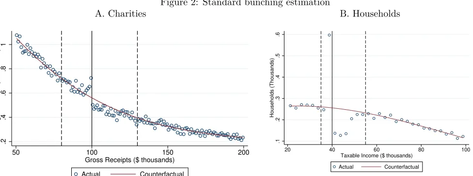
Visual examples of the standard approach are provided in Figure 2 for the charity and PSID datasets, respectively. In both figures, a polynomial is fit to the counts of income bin to estimate the counterfactual distribution, and mass is elevated in the bunching range just below the notch and reduced in the reduced range above the notch. Assuming no extensive-margin responses, the excess mass in the bunching range should equal the reduction of mass in the reduced range, and hence either of these can be used as the measure of bunching. Often this mass is divided by the counterfactual level of the density at the notch, and this bunching ratio gives an estimate of the amount by which the average buncher reduces income (Kleven and Waseem 2013).
3.2 Identification Challenges
Extensive-margin responses present one concern for static bunching estimation. The standard approach relies on the identifying assumption that in the absence of the bunching response there would be a smooth, continuous distribution of income in the neighborhood of the threshold of interest. If agents who would be above a notch are instead missing from the data, then this will reduce the mass found above the notch even if there is no bunching.
Some bunching papers have considered the nature of extensive-margin responses and how they might be detected or addressed. A point made by Kleven and Waseem (2013) and generalized by Best and Kleven (2018) is that there should be no such responses just above the notch when agents can simply bunch at very little cost relative to their preferred income level. This condition may not hold if frictions prevent bunching, as studied in much of the literature, or if exceeding the threshold causes attrition from the sample for reasons outside of the agents’ control, such as an increased probability of being audited and removed from the sample. Kopczuk and Munroe (2015) note that even when the result holds in the limit, extensive-margin responses may still occur close enough to the notch to affect estimation, and that it is not possible (with the standard bunching design) to measure extensive-margin responses without making strong assumptions. They suggest using only the data below the notch to estimate bunching and testing for the existence of extensive-margin responses by comparing the excess mass below to the reduced mass above. In this paper I measure the degree to which extensive-margin responses affect estimation, and I propose the first tool for estimating their extent.
in later years. This distortion can affect incomes far from a notch and therefore violate the identifying assumptions of static bunching estimation. In Appendix A, I mathematically demonstrate the issue for discrete and discrete-continuous distributions. Here I provide a visual example using the first ten years of earnings from each household in the PSID.10 To capture a situation without serially-dependent income I
simply impose bunching at the hypothetical $40,000 notch in each year. To capture serial dependence I construct another version of the panel in which I impose bunching in each year before applying the growth rates in the data to obtain potential income for the next year.
Figure 1 displays the distribution of income at different points in time. Panel A shows incomes at the 10-year horizon with and without serial dependence. With no serial dependence the distribution is, by construction, consistent with the expected features of bunching: there is a spike below the threshold, a trough above, and no distortion further from the threshold. The distribution with serial dependence also appears to have these features, indicating that it may not be obvious whether or not an empirical distribution has been influenced by serial dependence. By comparing this distribution to that without serial dependence, however, we can see that the mass is relatively high everywhere below the threshold and relatively low above it. This suggests the first diagnostic for researchers to evaluate, which is a “donut-RD” regression discontinuity design that excludes the bunching region and tests whether the estimated counterfactuals meet at the threshold. In the charity setting, annual RD estimates (not shown) reveal that the discontinuity in the distribution of income at the notch has grown steadily over most of the sample period, and annual bunching estimates fail to uncover this pattern. In Figure 1, Panel B shows how the difference between the two distributions emerges over time, with large differences emerging within five years in this example. Going beyond this example, the nature of this evolution will vary with the underlying dynamics.
For clarity, I will abstract from a variety of other potential complications with bunching estimation. For example, this paper focuses on empirics and will not discuss the challenges of interpreting bunching estimates in terms of the parameters of decision models (Einav et al. 2017, Blomquist and Newey 2017, Bertanha et al. 2018). For the sake of clarity, I have eschewed some adjustments that have been made to basic bunching estimation. For one, researchers have sometimes attempted to address complications such as income effects by estimating the counterfactual separately on either side of the threshold or adjusting the counterfactual above the threshold so as to equalize the excess- and reduced-mass estimates (e.g., Chetty et al. 2011). For another, the mass in a strictly dominated region just above the notch can be used to estimate the number of agents facing frictions that prevent bunching (Kleven and Waseem 2013). Optimization frictions have
10I make 300 copies of each household to increase the sample size and multiply initial income by a random number to
garnered increasing attention in the literature, and the methods proposed in this paper might find useful application in studying the nature of such frictions in both the short and long run. These adjustments can easily be incorporated into the dynamic designs in this paper, but I present versions without them to focus attention on the identification issues addressed by dynamic methods and the new parameters that these methods allow researchers to estimate.
3.3 Simulation
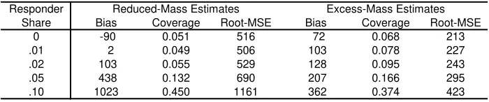
To examine the severity of this problem posed by extensive-margin responses I take 10,000 draws of 100,000 observations from the smoothed distribution of incomes in the PSID. I create a hypothetical notch at income of $40,000 and impose that no households bunch but that a fraction whose incomes fall above the notch are not observed. These missing observations represent responses on the extensive margin, and I vary the share of responding households between 0 and 10 percent. I estimate the average income foregone by bunchers using the standard, static approach. The response can be calculated using the estimates of either the excess mass below the threshold or the reduction in mass above the threshold, which should be equal absent extensive-margin responses, and I report the estimates from both approaches. Because the true amount of bunching is zero, the average estimate gives the bias, and the percentage of statistically significant results gives the coverage. I also report the root mean squared error (root-MSE).
Table 1 shows the effect of extensive-margin responses on static bunching estimates. Estimates using the reduced mass above the notch show small biases, as well as coverage rates close to 0.05, when 2 percent of the sample or less responds on the extensive margin. When these responses are more prevalent, the reduced-mass estimates falsely attribute them to bunching and reject too frequently. The pattern is similar for the excess-mass estimates, though these show inflated rejection rates even for small shares of extensive-margin responders. This may be surprising, given that the extensive-margin response occurs entirely above the notch and not in the bunching range. Even so, these estimates are biased because the reduced mass above the omitted range lowers the counterfactual mass within the omitted range, including below the notch.
Table 2 quantifies the bias in the static estimates arising from serial dependence of income. I impose bunching in the base year but estimate bunching in the next year when there is no bunching. I vary the degree of serial dependence by applying empirical growth rates to a weighted average of the preceding potential income and actual income. When the weightη on potential income is zero there is perfect serial dependence,
positive serial dependence (η <0), both estimates show a positive bias, and coverage rates rise rapidly. With
negative serial dependence (η >0), the bias in the excess-mass estimates becomes negative, while coverage
rates are again high for both estimates. Based on the graphical evidence in Figure 1, these biases would likely grow over time.
3.4 Application
Static bunching estimates for charities appear in Table 3.11 I use the sample of charities in years up to
2007 (before the notch was moved) that also appear in the prior year (for maximum comparability with the dynamic estimates that follow). The first row of the table shows estimates of excess mass below the notch. An estimate of .1 would indicate .1 percent of all charities in that year’s sample are below the notch and should be above it. The results from the basic specification indicate that the share of charities appearing below the notch is .148 percentage points greater than predicted by the counterfactual. In the second row this number is divided by the value of the density at the notch to give the bunching ratio, which can be interpreted as the average amount by which agents are willing to reduce income to bunch.12 The bunching
ratio is reported with the density in log scale, and it indicates that the number of bunching charities is roughly equal to the number of charities that should be above the notch by up to $600 (=$100,000*.00592). If all income responses are real (and not simply reporting responses), then this estimate would imply the average charity is willing to pay $600 to file Form 990-EZ instead of Form 990. The third row displays the estimated reduction of mass above the notch, which is nearly 70 percent larger than the estimate of the excess mass below.
The estimates in Table 3 raise the question of why the reduction in the number of charities above the notch is significantly larger than the increase in number below the notch. The “Basic” specification suggests the excess is only about 60 percent of the reduction, and the size of the reduction suggests charities may be willing to pay as much as $1000 to avoid Form 990. The second and third columns present the results of more flexible specifications motivated by regression discontinuity designs, but these do not reconcile the two results. The (“Discontinuous”) specification in the second column allows for a discontinuity at the notch. This reduces the estimate on both sides by a very small amount, leaving the asymmetry in the estimates. The (“Two-Sided”) specification in the third column estimates separate polynomials on each side of the notch. This gives a negative point estimate for the reduced mass, which would imply bunching in the range where mass should be reduced, and again failing to reconcile excess- and reduced-mass estimates.
11I use charities with receipts of $50-200,000 and a polynomial of degree 3, which minimizes the Akaike information criterion.
12With a homogeneous elasticity, there will be no mass in the missing range. With no extensive-margin responses, the reduced
These findings suggest the comparison of excess-mass estimates and reduced-mass estimates as a diagnos-tic. As noted above, Kopczuk and Munroe (2015) use this diagnostic to test for extensive-margin responses, then focus on the one-sided estimate of the excess mass. In the charity setting, the excess-mass estimate is more robust to the choice of specification in Table 3. However, as the simulations have shown, it may still be biased by serial dependence. I will provide further evidence of this by comparing the static estimate to the dynamic MLE estimate in Section 6. In settings for which a lack of panel data would make dynamic methods impossible, researchers can still compare the static excess- and reduced-mass estimates. Researchers should also be cautious about constraining estimation so as to require that the excess mass equal the reduced mass, as this equality need not hold in the presence of extensive-margin responses or serial dependence.
It should also be noted that the literature has done little to exploit panel data for heterogeneity analysis. It is straightforward to split a sample by pre-determined categorical variables, such as gender, and obtain static estimates for each subsample. It is less clear how to incorporate continuous and time-varying covariates into the static design. Some researchers have estimated the share of agents who remain in a bin over time, but slower growth by those in bunching bins could reflect either negative selection into current bunching or a greater likelihood of future bunching. A more dynamic approach is required to assess causation and to more fully exploit panel data to learn about heterogeneity in responses to the notch.
4 Dynamic Bunching Estimation: Temporary Notches
I now propose and evaluate designs that exploit panel data. I present these in order of abstraction from the static design. The design in this section makes a small adjustment that provides an alternative estimate of responses in the year of bunching. With panel data and a temporary notch, it also yields information about the dynamic effects of bunching. The design offers a test for serial dependence, which may provide evidence about whether bunching is driven by real income responses or misreporting.
4.1 Description of Method
The small adjustment I propose to the standard bunching estimate is to widen the bins to identify an unselected “treatment group” of agents with incomes near the notch. If the response to the notch is only local, then it will be possible to identify a range around the notch that includes all responders, i.e. that includes both the bunching range and reduced range. If one takes the entire omitted range as a bin, rather than using smaller bins on either side of the notch, then the sample within the bin is not selected because it contains both agents who respond and agents who don’t.
measured in logs, so that estimates can be interpreted as percentage changes.13 Let the bunching region
and reduced region have respective widthsωE andωR, and bins will now have widthωE+ωR. To simplify
notation, rather than denoting the maximum value in the bin,bini will now be defined by the bin straddling
the notch, withri∈(ρ−ωE, ρ+ωR]⇔bini =ρ⇔N earN otchi= 1. The following equation can then be
estimated with either cross-sectional or panel data.
ri=β·1[bini=ρ] + K X
k=0
αkbinki +ei (2)
As in Equation 1, the parameters αk describe the counterfactual distribution using a polynomial of order K. The parameterβ gives the average deviation from this counterfactual of the observations in the bin that
surrounds the notch.14
Identification is similar but not identical to that in the standard bunching design. Both rely on an identifying assumption that a polynomial can approximate a counterfactual function of bin level. Here, that function describes conditional mean income of agents in the bin, rather than the count of agents in the bin. Neither design’s assumption implies that of the other.15 Thus, researchers may wish to test robustness by
estimating bunching using both Equation 1 and Equation 2. Moreover, this approach becomes particularly useful with panel data and with a temporary notch that only exists in one period. Panel data make it possible to replace the outcome of Equation 2 with later years’ values of income (or other variables). A temporary notch simplifies interpretation because these later outcomes should not be affected by whether notch-year income was close to the notch unless the induced bunching in that year had persistent effects on these later outcomes. That is, if there is only a notch in the base year, then there should be no active bunching in the next year. A temporary notch also makes identification more credible because the treated group of agents with income near the notch should not be a selected sample, whereas a long-standing notch might have accumulated a selected sample of long-term bunchers. With panel data, researchers can test exogeneity of1 [bini=ρ]by estimating “effects” on outcomes determined before the year of the notch.
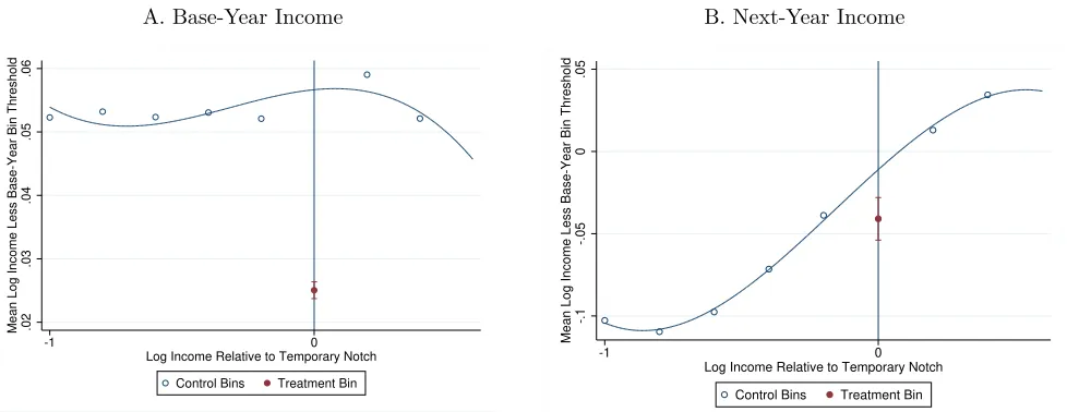
Figure 3 demonstrates how the approach provides an alternative estimate of bunching. In each panel, observations are binned by log income relative to the threshold in the base year, when the notch is imposed. As with the standard approach, I use data generated from the smoothed distribution of incomes in the PSID
13Static estimation can be performed with log income; this transformation does not account for the differences in results
between static and dynamic estimates.
14Diamond and Persson (2016) use a similar design to estimate long-run effects of test score manipulation by teachers. They
allow for a discontinuity in the counterfactual density; for simplicity and comparability with the standard estimator I assume a continuous counterfactual density.
15As a counterexample in one direction, suppose that income is uniformly distributed in all bins and that the bin count takes
and generate bunching at a notch at an income threshold of $40,000. Unlike the figures employed for the standard approach, which plot the counts in each of the bins, this figure displays conditional means. Panel A displays mean log income relative to a “bin threshold” that corresponds to the location of the notch in the treatment bin. Here the bin width is 0.2 and width of the bunching range is 0.05, so the bin threshold for each bin is a log income of 0.05 above the minimum log income in the bin.16 Panel A shows that bunching
in the (red) treatment bin has reduced its mean log income relative to the counterfactual mean predicted by surrounding bins. Changing the outcome of the regression to an indicator for having income above the bin threshold provides an estimate of the share of bunchers in the bin. The ratio of these two estimates should equal the average amount by which bunchers reduce income, the usual quantity of interest in bunching estimation.
The great advantage of this approach lies in the ability to estimate effects on future outcomes occurring after the notch is removed. Panel B of Figure 3 plots income in the year after the notch. Importantly, outcomes are again examined as a function of base-year income, which should not be influenced by the notch except in the treatment bin. For this illustration I have assumed perfect serial dependence, which implies that base-year bunchers’ incomes should be reduced one-for-one in the next year. Panel B of Figure 3 shows that this is the case, with next-year incomes reduced in the treatment bin by about the same amount that they were in the base year. Because having incomenear the notch in the base year was not endogenous to the notch, these figures show the causal effect of bunching on later income. Moreover, the treatment bin should have no effect on next-year income except through base-year income and can therefore be used as an instrument to estimate the degree of serial dependence in income. Additional outcomes can include functions of next-year income, including indicator variables for having income above the base-year bin threshold, above either of the minimum or maximum income levels in the bin, or in between the two.
4.2 Simulation
I perform two types of simulation to evaluate the temporary-notch design. First, I estimate bunching in base-year distributions in which there is no bunching. Second, I generate bunching in base-year distributions and estimate next-year outcomes, which I do for several degrees of serial dependence. For comparability with the corresponding static estimates I again use the smoothed distribution of annual taxable incomes from the PSID and draw 10,000 samples of size 100,000 for each of these simulations.
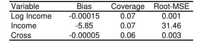
Table 4 quantifies the bias in the temporary-notch base-year estimates. The truth in this simulation is that there is no bunching, and hence all estimates should be close to zero. The results are as desired;
16The normalization of log income by subtracting the bin threshold level is irrelevant for estimation but makes the figure
on average, I estimate an income reduction of 0.017 percent, and the share of households in the treatment bin that bunch is 0.00033. The bunching ratio, which is expressed in thousands, indicates that the average household in the treatment bin reduces income by $6, in contrast with the static approach estimates in Table 2 that approach $1000 on average in some simulations. Coverage rates are also appropriate with roughly five percent of the estimates reject the true null of no bunching.
Table 5 displays the accuracy of the estimator under various degrees of serial dependence. Each cell of the table gives the average of the estimates for a particular outcome and simulation. The standard error in parentheses is the standard deviation of the estimates. As in Table 2 for the standard approach, I vary the weight of potential income relative to observed income. A weight of 0 indicates perfect serial dependence, 1 indicates no serial dependence, and 2 indicates that bunching households’ income rebounds in the next-year, as it would if base-year income was retimed. This weight is unrelated to the amount of bunching in the base year, and hence all base-year estimates of the reduction in income and share of households above the notch are similar. Moving to next-year outcomes, there should be no significant effects if there is no serial dependence, and this is indeed what I find when the weight on potential income is 1. With positive serial dependence (weight on potential income less than one), bunching has negative effects on next-year income. Conversely, with negative serial dependence (weight on potential income greater than one), bunching has positive effects on next-year income. Using the treatment-bin dummy as an instrument for base-year income provides an estimate of its effect on next-year income, and one minus this coefficient gives an estimate of the weight on potential income. The estimated weights are all slightly greater than the true weights, but they are all within one standard error of the true values.
The simulations provide evidence that the temporary-notch estimator has good properties. This approach can be used as an alternative to the standard approach in the cross-section, and with panel data it can be used to estimate dynamic effects.
4.3 Application
Variation in the IRS reporting notch for public charities makes it possible to estimate effects of a temporary notch. After decades with a notch at a nominal value of $100,000, the notch was moved to $1,000,000 for 2008, $500,000 for 2009, and $200,000 thereafter. The 2008 and 2009 notches were therefore only temporary (one-year) phenomena that should not have induced either repeated bunching or manipulation at incomes far from the level of the notch. I exploit this temporary nature, focusing on the 2009 notch, which fell at an income level affecting many more charities than the 2008 notch.
I estimate Equation 2 using 2009 log receipts as the binning variable.17 I examine three different functions
of income as outcomes. The first is simply income (log gross receipts), which is expected to be negatively affected in 2009 by the opportunity to bunch. The second, labeled “Cross 2009 Threshold,” is an indicator for whether an organization’s current receipts are above the level in its bin that correspond to the notch.18
Bunching should also have a negative effect on the probability that treated observations cross the 2009 threshold in 2009. Finally, I construct an indicator for current receipts that lie within the same bin that the charity occupies in 2009. This dummy takes the value of one for all observations in 2009 but provides another useful measure of pre-trends or long-term effects. Marx (2018) presents figures akin to Figure 3, and these provide visual support for the continuity assumption.
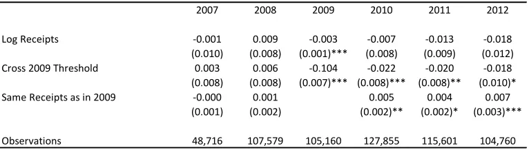
Results of the temporary-notch regressions for charities appear in Table 6. Each cell of the table reports the estimate of the parameterβfor a different outcome and year. In the first row the outcome is log receipts,
which is negatively impacted in 2009, as expected. The coefficient for this year implies that the average charity near the notch reduces log income by .003, i.e. reducing income by roughly $1500 ($500,000*.003). Estimated deviations from expectation are negative for subsequent years, but standard errors are large because in this setting (as will also be seen for the PSID), the distribution of year-over-year income growth has fat tails. The alternative income measures, which focus on more central moments, can therefore offer evidence that is more precisely estimated. In the second row, one can see that the probability of being above the notch in 2009 is reduced by 10.1 percentage points among the treatment group. These charities are not significantly different in this regard prior to 2009, but bunching in 2009 appears to cause a permanent 2 percentage-point reduction in the probability that treated charities ever achieve receipts greater than $500,000. Similarly, the third row shows that while these charities were no more or less likely to be in their year-2009 income bin in years before 2009, the probability that they remain in this bin (rather than growing out of it) is permanently increased by at least .4 percentage points.
Permanent effects of a temporary notch provide evidence of positive serial dependence of income. Marx (2018) discusses the apparent implication that manipulation in the charity setting was not entirely carried out by misreporting income. Here I will emphasize the implication, taking into account the simulation results in Section 3.3, that there is likely to be bias in static estimates of bunching at the repeated notch that was in place for all sample years before 2008. That the static estimates are biased is consistent with the evidence that follows.
greater than $100,000 to avoid lingering effects of the original notch, and log receipts bins of width .155, the width of the smallest omitted range that provides robust static bunching estimates. This approach is still potentially susceptible to extensive-margin responses, but for the temporary notch of 2009 this does appear to be a problem: the static estimate of excess mass below the notch is not statistically different from the static reduced-mass estimate or from the dynamic estimate obtained from the methodology described in Section 6, and the dynamic estimate of extensive-margin responses is not significantly different from zero.
18This dummy variable indicates that the charity has receipts greater than .065 plus the level of the minimum income in the
5 Dynamic Bunching Estimation: Ordinary Least Squares
Esti-mation
This section describes another easily-implemented dynamic extension of the ordinary-least-squares binning approach to bunching estimation. This extension can be applied to settings in which a notch is faced repeatedly. Serial dependence is addressed by conditioning on past income.
5.1 Description of Method
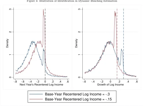
Consider agents observed in a base year and the next year, with a notch existing in the next year and possibly the base year as well. Figure 4 depicts such a situation using the smoothed PSID distribution. Panel A of the figure shows the distribution of log income in the next year for two illustrative levels of base-year income. Because modal growth is roughly zero, each conditional distribution of next-year income is centered around the level of current income. For each group, the distribution of next-year income is distorted around the notch as one would expect, with excess mass just to the left and reduced mass just to the right. Panel B shows the distribution of growth rates for each group. Because income is logged, the growth rates are a simple translation of the group’s next-year income that subtracts base-year income.
Panel B of Figure 4 conveys the intuition for a dynamic bunching estimation identification strategy. Households with different levels of base-year income have similarly-shaped growth distributions, except that each has a bunching distortion at growth rates that would take the household close to the notch. Because the depicted groups are starting from different income levels, each approaches the notch at a different level of growth, and hence the distortions lie in different parts of the two groups’ growth distributions. The extent of the distortions can therefore be estimated by comparing the shape of one group’s growth distribution around its notch to the corresponding, undistorted section of the growth distribution among households in the other group. This insight can then be extended from two levels of base-year income to all levels, with each providing a counterfactual distribution for the rest.
The dynamic bunching identification strategy can be implemented in a variety of ways. In theory, one could estimate the entire multivariate density of income in all available years, but allowing for such generality would be computationally expensive. I propose two implementations that focus on pairs of base-year log income (rit) and growth to next-year income (git=rit+1−rit). Section 6 presents an implementation using
and control groups for a permanent notch in much the same way as for a temporary notch, as described in Section 4. Also like the temporary-notch approach, outcomes of interest will be means of income or growth conditional on falling within each bin.
To develop intuition before considering the full OLS implementation, consider restricting a dataset to agents’ whose growth rate from any base year to the next year falls within a particular range. As an illustration using the empirical application, Figure 5 plots the mean growth rate by bins of base-year income. The sample includes all observations of charities growing log income by .1 to .2 between the base year and the next year. For some bins of base-year income, this range of growth implies next-year income that is near the notch but mostly or entirely to one side of it; these bins may therefore include a selected sample of bunchers or non-bunchers, and hence they are depicted with light gray markers and excluded from estimation. However, for the bin with base-year income between −0.18 and −.013, growth of .1 to .2 translates to a
range of future income that straddles the notch. Thus, agents in this bin should provide a sample that is not selected based on whether an agent would bunch. This bin can therefore be labeled as the group treated with the opportunity to bunch, as in the temporary-notch estimation. It is represented in the figure by the filled circle with standard error bands. Empty circles display the growth rates of charities with higher or lower base-year income, and the curve with standard error bands illustrates a quadratic fit to these control bins. The interpolated counterfactual implies that average growth, conditional on growth in the range of .1 to .2, should be nearly .147 for charities nearing the notch, but the estimate for this group is instead less than .145. The difference provides an estimate of the effect of nearing the notch on observed income.
A more general design incorporates multiple ranges of growth rates by stacking estimates for each ofγ
different growth-rate bins of widthωg and maximum value labeledgbinit of equal width. Again, denote by ritagenti’s log income in base yeart, and label the growth rate to the next year’s income git=rit+1−rit.
Bins of base-year income can be selected with widthωrand maximum value labeledrbinit. To estimate the
effect of nearing the notch on outcomeYit+1, I propose estimating equations of the form
Yit+1=β·N earN otchit+ K X
k=0
X
γ
αkγrkit·1[gbinit=γ]. (3)
Here, the “treatment” variable isN earN otchit=1[rbinit−ωr+gbinit−ωg< ρt+1< rbinit+gbinit], which
indicates pairs of income and growth-rate bins that produce a range of next-year income that straddles the notch ρt+1. As in previous methods, the α coefficients describe the counterfactual, which now varies in
two dimensions by allowing for a separate polynomial of base-year income for each bin of growth. As in temporary-notch estimation,β gives the difference between the conditional mean of the outcome and what
β <0. Note that base-year characteristics should not be affected by nearing the notch in the next year, and
hence interactions with these characteristics can be used to describe heterogeneity in the bunching response, even if these characteristics are continuous variables.
Appendix B provides additional details. As Figure 5 indicates, some care is required in constructing the treatment bins and choosing omitted bins. In the Appendix B propose the use of bin count as an outcome to test the exogeneity of the treatment bin. I also describe the construction of a useful outcome variable that provides a direct estimate of the share of agents who bunch.
5.2 Simulation
I evaluate the dynamic OLS approach with the same type of simulations used for the static and temporary-notch approaches. Using the smoothed PSID income distribution, I generate 10,000 random samples of 100,000 observations in each. I induce bunching at the hypothetical notch at base-year income of $40,000, then apply an observation’s growth rate to its (potentially bunching) base-year income to obtain next-year income. I then estimate bunching in next-year income, for which the true value is zero, and examine the bias, mean squared error, and coverage rates.19
Table 7 presents the results of the dynamic OLS simulation. The first row presents results for log income, which would be reduced in the treated bins approaching the notch if households in these bins chose to bunch. The coverage rate is close to 0.05, and the bias and root-MSE are very small. These magnitudes can be evaluated more easily for levels than for logs because the static estimates offer a comparison in levels. The second row of the table transforms the estimates to levels by exponentiating the direct estimates, which changes the bias and root-MSE but not the coverage rage. The relevant comparison among the simulations of static estimation is the top row of Table 2, in which the setup is identical because serial dependence is perfect. Compared to the dynamic OLS estimates, the excess-mass static estimates (which performed better than the reduced-mass estimates) have a coverage rate this is three times larger, root-MSE that is nearly 8 times larger, and absolute bias that is 2000 times larger. Moreover, the dynamic approach provides a direct estimate of the effect of approaching the threshold on the probability of crossing it. The last row of Table 7 shows that for this outcome the absolute bias is half of one percentage point, and the coverage rate is less than 0.06.
19The estimation uses base-year log-income bins of width 0.05, growth rate bins of width 0.1, and an omitted range of base-year
5.3 Application
Dynamic OLS estimation can be performed with nearly the same ease as static estimation, and it can offer several improvements. For one, it can address the identification issue posed by serial dependence, as shown by the simulation. Another benefit is the opportunity to study heterogeneity in agents’ responsiveness to the notch, particularly when this heterogeneity relates to time-varying characteristics. Such characteristics can be made time-invariant, such as by defining them as having their value in the base year, and then interacting them with the treatment-group dummy and potentially other variables. Using this approach, Marx (2018) estimates that the responses of charities to the reporting notch are related to both size and staffing, providing evidence describing the nature of the compliance cost and induced avoidance behavior.
Here I focus on the effect of the notch on long-run growth, which also cannot be estimated with the standard design. The last row of Table 7 showed simulation results for a binary outcome indicating growth exceeded that required to be above the notch at timet+ 1. Corresponding indicators can be defined for any
horizon hto estimate effects of approaching the notch at timet+ 1on crossing it at timet+h. 20 Table
8 displays the results of regressions with h varying from 1 to 12.21 For charities in the bins approaching
the notch in yeart+ 1, the estimated counterfactual is that 40 percent should have income greater than the
notch att+ 1, and 75 percent should have income above the notch in yeart+ 10. The estimates in the table
suggest that bunching reduces these probabilities in both the short- and long-run. I find the largest effect, a 5.3 percentage point reduction, in the year that the notch is first approached. I then find effects of around 1.5 to 2 percentage points at all other horizons, implying that the notch permanently reduced the growth of a significant number of charities.
6 Dynamic Bunching Estimation: Maximum Likelihood
Estima-tion
Dynamic OLS estimation is straightforward and provides a number of potential advantages over static OLS estimation. However, as in static bunching estimation, this design will not account for extensive-margin responses without additional assumptions. Moreover, the OLS estimates are unlikely to be efficient because binning the data treats observations within a bin as equivalent, and throughout the literature, the choices of bin widths and locations have been ad-hoc. To address these limitations, I now propose a maximum
20For the group withN earN otch
it= 1, this outcome indicates exceeding the level of growth that would be required to cross
the notch att+ 1. For those withN earN otchit= 0it indicates a corresponding growth rate depending on position in the bin
of base-year income.
21Counterfactual estimated as a quadratic function of current receipts, controlling for growth-rate bins of width .1. The
likelihood bunching estimator.
6.1 Description of Method
Dynamic bunching estimation with MLE retains the flexibility of OLS estimation. This is because identifi-cation is obtained by comparing parts of the joint distribution of income in multiple years, as was described in Section 5 and depicted in Figure 4. OLS estimation involves choosing a functional form (the polynomial) and then adding parameters as needed to flexibly fit the data. MLE estimation proceeds similarly, starting from a functional form that reflects the fact that the researcher is estimating a probability distribution.22
As before, rit is a agent i’s log income in a base-yeart, and growth to the next year isgit =rit+1−rit. A
researcher can first choose a functional form with parametersΘforF∗(git|rit,Θ), the latent cdf that would
be observed if no observations were bunching or going missing from the data. Bunching and extensive-margin parametersΩcan then be incorporated to construct the distributionF(git|rit,Θ,Ω)that is fit to the data.
Laplace (or “double exponential”) distributions offer a natural choice for the basic form ofF∗(git|rit,Θ).
These distributions have been used extensively to model financial data and are described by Kotz et al. (2001) as “rapidly becoming distributions of first choice whenever ’something’ with heavier than Gaussian tails is observed in the data.”23 I estimate a flexible version of the Laplace cdf by allowing for flexible functions Pl(g, r,Θ)andPu(g, r,Θ) to enter the lower and upper pieces of the distribution:24
F∗(git|rit,Θ) =
exp(Pl(git, rit,Θ)) git< θ
1−exp(Pu(git, rit,Θ)) git≥θ
, (4)
where θ is a location parameter that I set equal to zero based on the shapes of the distributions in both
datasets. Appendix B motivates the focus on the cumulative distribution function and provides details of the specification and implementation, including derivation of parameter restrictions that for flexible choices of
Pl(g, r,Θ)andPu(g, r,Θ)while ensuring that the resulting function satisfies the properties of a probability
distribution. R code for implementation is available online.
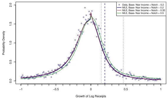
Figure 6 provides a visual example using draws from the smoothed PSID distribution. The figure focuses on illustrative base-year log income level of 0.2 less than the hypothetical notch at log($40,000). The
empirical density of growth rates conditional on this level of receipts (and others) is non-Normal, with a sharper peak around zero growth and fatter tales, motivating the use of a Laplace distribution, as in
22Kopczuk and Munroe (2015) use MLE to estimate bunching within the static framework.
23See Kozubowski and Nadarajah (2010) for other applications.
24The symmetric Laplace distribution with location parameter θand scale parameter σ has this form with P
l(g, r,Θ) = Pu(g, r,Θ) =
g−θ
σ
Equation 4. It is also not well approximated by the basic, two-parameter Laplace distribution, requiring higher-order functions forPl(git, rit,Θ)andPu(git, rit,Θ). The estimated functions, listed with other details
in the following Subsection on simulation, provide a counterfactual (dark curve) that approximates the PSID distribution (circular markers). The notch for this level of base-year income occurs at a growth rate of 0.2, and the omitted range is drawn around this. Using two other illustrative levels, the figure also displays how the counterfactual varies with base-year income.
Responses to the notch are estimated by maximizing the likelihood of the observed data according to a censored version,F(git|rit,Θ,Ω), of the latent distributionF∗(git|rit,Θ). The added parametersΩdescribe
bunching and attrition. The censoring occurs in the omitted region, which varies withrit, as depicted for one
level ofritin Figure 6. F∗(git|rit,Θ)determines the probabilities, for a given level ofrit, that an observation
will appear in its bunching region or reduced region. Outside of this region, one can use the pdf derived from F∗(g
it|rit,Θ). Attritors can be assigned a specific, fill-in value of git, and then attrition can also be
estimated with censoring. For example, in the simulation I treat all attritors as havingrit+1=log(10,000),
with correspondinggit, and then estimate a probability mass for this level ofgitthat can vary with rit and git. In this way, I capture extensive-margin responses of households whose next-year income would exceed
the notch-level growthρitif they were observed. I do so by incorporating a parameter that shifts mass from
(1−F(ρit|rit,Θ))toP r(rit+1=log(10,000)).
6.2 Simulation
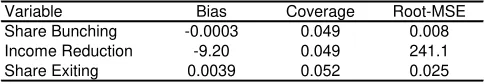
The simulation of MLE dynamic bunching estimation follows the earlier simulations. Again, observations are generated from the bivariate PSID distribution. I draw 10,000 random samples of 10,000 observations, a smaller sample size because the time required to obtain each MLE estimate is many times that for the OLS estimates. As in previous simulations, I impose bunching in the base year but no bunching or notch-related extensive-margin responses in the next year. I randomly select observations to attrit at a rate of about four percent, matching the attrition rate among high-income households in the raw data. I estimate extensive-margin responses of households that should cross the notch (as in the application below). I also allow for attrition that is a flexible function of base-year income.25
Table 9 presents results from the simulation. I report estimates describing bunching and extensive-margin responses, both of which have a true value of zero. The top row describes estimates of the share of bunchers among the total number of households that should move to the reduced region. The second row reflects the
25Estimation uses base-year log incomes within 0.5 of the notch at log(40,000)≈10.6, with omitted range of next-year log
incomes of 10.5 to 10.9. The flexible functionsPl(git, rit,Θ)andPu(git, rit,Θ)include a number of subfunctions ofgit, each
multiplied by a quadratic function of base-year log income. These subfunctions are quintic, exponential, and the arc-tangents
estimated effect on the income of these households, and the third row represents estimates of the percentage of those that should cross the notch that instead exit the sample. Despite the imperfect specification of the counterfactual, as seen in Figure 6, all of these estimates exhibit a bias close to zero and a coverage rate close to 5 percent.
6.3 Application
For the charity application, I estimate functions similar to those used for the simulation.26 The latent
distributions are similar to the PSID distributions in Figure 6, but attrition is more common in the charity data. Attrition could be due to late filing, earning income below the level at which filing is required, shutting down, merging, or simply failing to comply with the reporting requirement. I estimate types of attrition that vary withrit and may or may not be systematically related to the notch.27
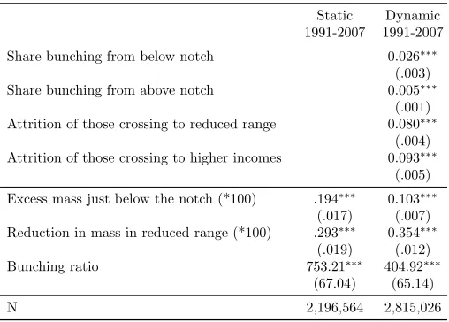
Table 10 displays maximum likelihood dynamic bunching estimates. The first column provides static bunching estimates for comparison with the dynamic bunching estimates in the second column. The top panel of Table 10 shows estimates of parameters governing bunching and systematic attrition. The first parameter gives the bunching propensity among charities that have base-year receipts below the notch. An estimated 2.6 percent of the charities that should enter the reduced range from below are instead bunching. The second row shows this bunching propensity is lower for those with current receipts above the notch (who have already filed Form 990 in the base year).
The third and fourth rows in the table show that attrition is systematically related to the notch. The estimated parameters indicate the share of charities that should be crossing the notch from below but instead go missing from the sample. This is estimated separately for those that would have entered the reduced range and those that would have grown to a point further above the notch. These estimates turn out to be similar and highly significant, revealing extensive-margin responses by 8 or 9 percent of charities that should cross the notch. Comparing the attrition and bunching propensities, a combined 10.6 percent of charities avoid filing when first crossing the notch to the reduced range, and the number of charities doing so by bunching is dwarfed by the number responding on the extensive margin. The static approach provides no such estimates of these extensive-margin responses.
The lower panel of Table 10 reveals the estimated excess share of charities below the notch and reduction
26The charity notch occurs atρ=log(100,000)≈11.51, and I include in the sample all observations with r
it <14. The
omitted range of next-year log incomes is(log(95,000),log(130,000)). The flexible functionsPl(git, rit,Θ)andPu(git, rit,Θ)
again include a number of subfunctions ofgit, each multiplied by a quadratic function of base-year log income. These
subfunc-tions are linear, exponential, the exponent of the square, and the arc-tangent. The argument of the arctangent is also multiplied
by a quadratic function of base-year log income. I adjustF(git|rit,Θ,Ω)to account for truncation of the sample due to the
fact that agents with income below $25,000 do not have to report.
27Baseline attrition is estimated as a quadratic function ofr
it. I allow this attrition rate to have additional slope and intercept
terms forrit > ρ. As explained in the description subsection for this method, I also estimate extensive-margin responses of
in the share above it. The excess and reduction are found by aggregating the bunching and attrition propensities across all observations in the base year according to their counterfactual probability of moving to the reduced region in the next year. The dynamic estimates of the share of charities that appear in the bunching range exceeds by .103 percentage points (or roughly 200 charities per year) the quantity that would have been found in the absence of a response. Consistent with the difference in estimated magnitudes of the propensities to bunch or leave the sample, the reduction of mass in the range just above the notch is significantly greater at .366 percentage points. Applying the static approach gives estimates of the excess and reduced mass that are much closer to each other, and both are significantly different from the dynamic estimates. Finally, the bunching ratio gives the ratio of excess bunching mass to the counterfactual density at the notch, here reported for the density in levels so that the ratio can be interpreted as a dollar amount. This ratio gives an estimate of average willingness to forego income to bunch, and as with the non-normalized excess-mass estimates, the result of static estimation appears to be biased upward by a factor of nearly two. Finally, Figure 7 provides a depiction of the difference between the two estimation approaches. The figure plots the density of receipts in the next year and estimated counterfactual densities. The MLE counterfac-tual is what Kleven and Waseem (2013) refer to as “a ’partial’ counterfaccounterfac-tual stripped of intensive-margin responses only.” Due to serial dependence of income and extensive-margin responses, the counterfactual is not smooth at the notch. That is, even if charities did not bunch in these years, the density would not be a smooth function of income as assumed in the static approach. The static approach estimates a smooth curve connecting the discontinuous pieces of the density, and as can be seen in the figure, this will underestimate the density below the notch and therefore overestimate the excess mass in the bunching region. Also, because the density is reduced everywhere above the notch, treating it as unaffected by the notch assumes away some of the true reduction above the reduced range and so underestimates the reduction in the reduced range. The figure shows that static bunching estimation conflates multiple responses, including repeated bunching and extensive-margin responses, and is not directly informative of the underlying behavior.
7 Conclusion
preference heterogeneity, long-run effects of approaching a notch, and the effect of bunching in one year on income in subsequent years.
Data analysis suggests a number of diagnostics that researchers can use to test for potential bias in static bunching estimates. Researchers studying notches can, even with only a single cross section of data, perform a statistical test of whether the excess mass to one side of the notch equals the reduction in mass on the other side. This test can be generalized by estimating the counterfactual distributions separately on each side of the notch (Kopczuk and Munroe 2015). With repeated cross sections, the researcher can examine whether bunching or donut-RD estimates vary by year, and in particular whether mass accumulates or discontinuities grow over time. With panel data, the researcher can compare the static and dynamic OLS estimates to assess whether estimation with dynamic MLE appears warranted. Finally, with a temporary notch, the researcher can estimate the degree of serial dependence in income.