Munich Personal RePEc Archive
Hedging under square loss
Bloznelis, Daumantas
Research Centre for Operations Research and Business Statistics,
KU Leuven, School of Economics and Business, Norwegian
University of Life Sciences, Department of Business Administration,
Inland Norway University of Applied Sciences
21 December 2017
Online at
https://mpra.ub.uni-muenchen.de/86708/
Hedging under square loss
Daumantas Bloznelis
1Research Centre for Operations Research and Business Statistics
KU Leuven
&
School of Economics and Business
Norwegian University of Life Sciences
&
Department of Business Administration
Inland Norway University of Applied Sciences
First version: April 18, 2016
This version: May 14, 2018
Work in progress – comments welcome
1 Mailing address: Høgskolen i Innlandet, Avdeling for økonomi- og ledelsesfag, Postboks 104, 2451 Rena,
2
Abstract
The framework of minimum-variance hedging rests on a restrictive foundation. This study shows that
the objective of variance minimization is only justifiable when variance coincides with expected
squared forecast error. Nevertheless, the classical framework is routinely applied when the condition
fails, giving rise to inaccurate risk assessments and suboptimal hedging decisions. This study proposes
a new, improved framework of hedging which relaxes the condition at no tangible cost. It derives a
new objective function, an optimal hedge ratio, and a measure of hedging effectiveness under square
loss. Their superior performance is demonstrated from a theoretical standpoint and by applying them
to hedging the price risk of oil and natural gas. Simple yet general, the new framework is well suited
to replace the classical one and facilitates adequate risk measurement and improved hedging
decisions. It also provides fundamental insight into dealing with uncertainty under square loss and
beyond.
(JEL: D81, G11, G32, Q02)
Keywords: minimum-variance hedging, hedging effectiveness, optimal hedge ratio, risk, uncertainty,
3
1. Introduction
Hedging is a classical means of risk reduction in financial markets. It exploits the idea that negative
surprises in the future price of an asset can be mitigated by investing in related assets with opposite
shocks. The future price of a portfolio formed this way is more certain than the future price of the
original asset. A popular measure of risk or uncertainty associated with price is its variance. Variance
measures the spread of a random variable around its expected value and hence is a natural and
appropriate measure of risk under square loss provided that the expected value is known.2 This
underlies the classical framework of minimum-variance hedging due to Johnson (1960) and Stein
(1961) and motivates the use of relative reduction in variance as a measure of hedging effectiveness
suggested by Johnson (1960) and Ederington (1979).3
However, financial variables such as share or commodity prices do not have known expected
values, rendering variance an inappropriate measure of risk under square loss (or any other loss
function). Indeed, a variable with zero variance but unknown expected value is in principle less
predictable and may produce more uncertainty than a variable with a known expected value and
moderate variance. This undermines the use of variance as a risk measure, and variance minimization
as a proxy for risk minimization. Employing variance as a risk measure in absence of a known
expected value may result in grave miscalculation of uncertainty and inferior hedging decisions,
particularly in short hedging horizons and for prices that have a predictable component, as will be
illustrated below both theoretically and empirically. Therefore, a replacement risk measure is
needed.
In general, our uncertainty over an outcome of a random variable is characterized by the
distribution of the difference between our beliefs, or our prediction of the value to be realized, and
2 An alternative term for square loss is quadratic loss.
3 The discussion of risk and uncertainty can be phrased either in terms of price or of return (i.e. price change).
The two formulations are mathematically equivalent and yield identical implications in the present context.
4 the actual random variable. Under square loss, this uncertainty is reflected by the expected squared
forecast error, a measure that applies regardless of whether the expected value of the random
variable is known or not. As such, the expected squared forecast error is a valid substitute for
variance for measuring hedging effectiveness under square loss.
The purpose of this paper is twofold. First, it is to identify, expose, and illustrate the problems
with the classical minimum-variance hedging framework in financial markets, and to relate them to
several of their symptoms known from the past. Second, it is to introduce a new, appropriate
framework of hedging under square loss based on minimizing the expected squared forecast error.
The new framework consists of a new objective function, an optimal hedge ratio, and a measure of
hedging effectiveness, all seamlessly generalizing their classical counterparts due to the
minimum-variance framework.
The new framework will primarily benefit hedgers by enabling them to properly measure risk
and adequately assess and compare the performance of alternative hedging strategies, allowing for
optimal hedging decisions to be made. It will also facilitate policymakers’ better understanding of risk
management and may lead to improved regulations and incentive schemes favoring efficient
strategies of uncertainty reduction. Therefore, current users of the classical minimum-variance
hedging can only gain from adopting the new framework, avoiding the pitfalls inherent in the
classical one.
The remainder of the paper is structured as follows. Section 2 reviews measuring uncertainty in
general and under square loss in particular. Section 3 presents the minimum-variance hedging
framework and traces some of its problems identified in the literature. Section 4 introduces the new
framework of hedging under square loss. Two special cases are considered in Section 5; one where
the expected values of prices are known and are used as point forecasts, and another where the
expected values are additionally known to equal the current prices. Section 6 provides empirical
5 and the adequacy of the new one. A conclusion and a discussion of the broader implications of the
main results are supplied in Section 7.
2. Measuring uncertainty
2.1 Uncertainty and the forecast error
Hedging pertains to reduction of uncertainty, and thus it is important to clearly delineate the latter.
Uncertainty reflects an agent’s lack of knowledge about the future price of an asset. It involves two
basic building blocks, the agent’s beliefs about the future price (formulated as a point or a density
forecast) and the future price itself (a random variable). The gap between the two, i.e. the mismatch
between the beliefs about the random variable and the actual properties of the variable, or the
distance between the forecast and the target, characterize uncertainty. Hence, uncertainty cannot be
defined without a reference to beliefs held by the agent facing it. For example, information on the
future price alone is not sufficient to characterize uncertainty if the information on the agent’s beliefs
(her forecast) is missing. Therefore, any definitions and/or measures of uncertainty based solely on
the price itself, such as its variance, are ill conceived. In contrast, relevant definitions and/or
measures of uncertainty reflect the discrepancy between the beliefs and the reality, hence, the
forecast error.
An agent cares about what the price of an asset will be in the future, but she does not know it,
hence the uncertainty. Currently, at time , the price of the asset is . In the future, at time + ℎ,
where ℎ > 0, the price will be . At time , the agent does not know , but she has some idea
of what it could be. She may have a density forecast or at least a point forecast for . Let us
consider the point forecast and let us denote it ̂ | , indicating that it is a point forecast of
made at time .
The difference between the actual realization of the future price and the forecast constitutes a
forecast error | ≔ − ̂ | . The error is realized (becomes known) at time + ℎ; before
6 in characterizing the price uncertainty that the agent is facing at time . These properties allow us to
investigate the uncertainty from a quantitative perspective, to measure it, and to link the practical
interpretation of uncertainty with its mathematical characterization.
Any and all probabilistic properties of | , including those characterizing uncertainty, can
be extracted from the probability distribution function and the probability density function of
| . For example, if large (negative and/or positive) errors are relatively likely to be realized, i.e.
their probability density is high, then the uncertainty is high. If large errors are unlikely, i.e. their
probability density is low, the uncertainty is low. Conversely, high uncertainty means that large
(negative and/or positive) errors are relatively likely to be realized, i.e. their probability density is
high. Meanwhile, low uncertainty means that such errors are unlikely, i.e. their probability density is
low. This is how the probability distribution of | is interpreted in terms of uncertainty, and
also how the practical understanding of uncertainty translates into probabilistic statements about
| .
2.2 Moments that reflect uncertainty
However, it is not always convenient to work with the probability distribution function or the
probability density function of a random variable. Instead, some summary characteristics may be
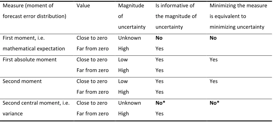
simpler to handle yet still serve the purpose of characterizing uncertainty; see Table 1 for a schematic
overview. For example, one such characteristic is the first absolute moment E | , where
E ∙ denotes the mathematical expectation conditional on the information available at time . When
E | is large, the probability density of large (negative and/or positive) errors must be high
and hence the uncertainty is high; when E | is small, the probability density of large errors
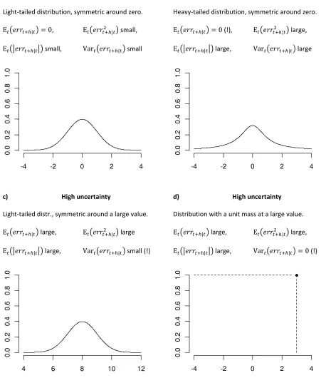
must be low and hence the uncertainty is low; Figure 1 illustrates the point. Conversely, high
uncertainty translates into high probability density of large errors and thus large values of
7 small values of E | . Thus E | is informative of the magnitude of uncertainty and
in general is a sensible measure of uncertainty.
[Table 1 about here]
[Figure 1 about here]
Another example is the second moment E | . When E | is large, the
probability density of large errors must be high and hence the uncertainty is high; when E |
is small, the density must be low and the uncertainty too. Conversely, high uncertainty and the
corresponding high probability density of large errors produce large values of E | ; and low
uncertainty produces small values. Just like the first absolute moment, also the second moment is
informative of the magnitude of uncertainty and thus is a sensible measure of uncertainty. Whether
to use the first absolute moment or the second moment depends on the loss function that is relevant
for a particular application. The first absolute moment is applicable under absolute loss, while the
second moment applies under square loss. Other summary characteristics of the probability
distribution, such as value at risk or expected shortfall, are relevant under other loss functions.
2.3 Moments that fail to reflect uncertainty
Not all summary characteristics of the error distribution adequately reflect uncertainty. That is, some
or all values of these characteristics are not informative its magnitude. The first moment, or the
mathematical expectation E | , is the simplest example. If E | is large (negative or
positive), the uncertainty is high, because a large E | implies that large errors are relatively
likely to be realized and that large positive errors do not outweigh large negative errors nor the other
way around. But if E | is small (close to zero), the uncertainty may be either low or high.
E.g. the error distribution may be light-tailed and symmetric around zero, which corresponds to low
probability density of large errors and hence low uncertainty; see panel a) of Figure 1. Alternatively,
the error distribution may be heavy-tailed and symmetric around zero, indicating high uncertainty
8 compatible with both low and high uncertainty, it is not informative of the magnitude thereof.
Hence, E | is not a sensible measure of uncertainty.
A similar case can be made for the second central moment, or variance Var | ≔
E | − E | . When it is large, large errors (either negative or positive, or both,
depending on E | ) are likely and the uncertainty is high; an example is provided in panel b)
of Figure 1. But if variance is small, the uncertainty may be either low or high. E.g. the error
distribution may be light-tailed and symmetric around zero, which corresponds to low probability
density of large errors and hence low uncertainty; see panel a) of Figure 1. On the other hand, the
error distribution may be light-tailed and symmetric around a large value (either negative or
positive), indicating high uncertainty because large errors are likely; refer to panel c) of Figure 1. A
more extreme stylized example is also possible and is depicted in panel d) of Figure 1. There, variance
is zero, i.e. the smallest possible, but the error distribution has all of its mass concentrated at a large
positive value, meaning high uncertainty because large errors are guaranteed. In summary, small
variance is perfectly compatible with both low and high uncertainty, and thus it is not informative of
the magnitude thereof. Hence, variance is generally not a valid measure of uncertainty.
Since the second moment is the sum of variance and squared first moment, variance of the
forecast error reflects forecast precision (the spread of forecasts around their center) but not
forecast accuracy (the closeness of the center of the forecasts to the target). Low uncertainty
requires high precision and high accuracy simultaneously, but low variance only ensures the former.
Using variance of the forecast error as a measure of uncertainty is akin to drawing the bullseye right
at the center of all shots after they have been fired. Clearly, this is not an adequate measure of the
overall skill of the shooter.
However, there is one condition under which variance becomes a sensible measure of
uncertainty; this condition is that the mathematical expectation be zero. In the context of forecast
9 precision). If the expectation is zero, variance equals the second moment: E | = 0
⇒ Var | = E | . Since the second moment adequately reflects uncertainty, the
expectation being zero ensures that variance does, too. The expectation being zero is an important
special case in which variance turns from an otherwise invalid measure of uncertainty into a valid
one; it happens, as variance becomes the second moment. Consequently, for all practical purposes of
measuring uncertainty, it is always safer and simpler to use the second moment in place of variance.
First, if the two coincide, there is no loss in using the second moment. Second, if they do not
coincide, it is only the second moment that appropriately measures uncertainty while variance does
not.
3. Minimum-variance hedging and its problems
3.1 Minimum-variance hedging framework
Minimum-variance hedging is one of the oldest and most popular approaches to hedging, introduced
by Johnson (1960) and Stein (1961).4 According to Johnson (1960), ““price risk” can be considered a
reflection of the variance <…> of a subjective probability distribution (or a subjective probability
density function) for price change from " to <…> where actual price from " to is treated as a
random variable”. This gives rise to declaring variance minimization the hedger’s objective:
Var # = E # − E # → min( , (1)
where # = # * = − *+ is the price of the hedge portfolio , = − *-; is the price of the
original asset ; + is the price of the hedging instrument -; and −* is the portfolio weight of the
hedging instrument; * is also known as the hedge ratio. The (negative of the) hedge ratio reflects the
hedger’s exposure to the price of the hedging instrument as a fraction (or a multiple) of the exposure
to the price of the original asset.
4 Historically, the role and definition of hedging has been investigated in numerous papers, e.g. Hardy and Lyon
10 Johnson (1960) and later Ederington (1979) suggested assessing hedging effectiveness by
calculating the relative reduction in variance due to hedging,
RRV , # ≔Var Var− Var # = 1 −Var #Var , (2)
where the absolute reduction in variance due to hedging, Var − Var # , is measured as a
fraction of the variance of the original asset, Var , to arrive at the relative reduction in
variance RRV , # . The higher the relative reduction in variance, the higher the effectiveness.
The final element to complete the minimum-variance hedging framework is the optimal hedge
ratio, *∗,01 (where the subscript ℎ indicates the hedging horizon and 34 stands for minimum
variance), which is defined as the argument minimizing the objective function,
*∗,01≔ arg min( Var # . (3)
The triplet {objective, optimal hedge ratio, effectiveness measure} constitutes the hedging
framework.
3.2 Problems with minimum-variance hedging
Johnson (1960) acknowledges that his concept of risk is different from traditional theory since it is
based on subjective rather than objective probability. He introduces a measure of hedging
effectiveness that is also defined in terms of subjective probability and does not account for the
actual distribution nor the actual realizations of price. However, the minimum-variance hedging
framework has been repeatedly employed with (estimated) objective probabilities in settings where
the price distribution and particularly the expected value (the first moment of the distribution) may
be unknown to the agent. This has led to numerous puzzling results and apparent paradoxes in the
literature.
Lien (2008) notes that persistent confusion permeates the literature on minimum-variance
hedging and on measuring hedging effectiveness. He observes that the empirical findings are often
counterintuitive. Multiple authors (Lindahl, 1989; Lien, 2005a; Alexander & Barbosa, 2007) state that
11 on the price changes, or returns5, of the original asset and of the hedging instrument. Lindahl (1989)
identifies a problem with using the classical measure when there is predictable development of the
basis, i.e. of the difference between the price of the original asset and that of the hedging
instrument. According to her, focusing exclusively on the unexpected changes in the basis would
yield a more precise definition of basis risk. However, she acknowledges that distinguishing between
expected and unexpected changes is difficult and therefore does not apply this idea in her work. Lien
(2005a) identifies a mismatch between the aim of minimizing the conditional variance of portfolio
returns when estimating a model in sample and the evaluation of the model performance by
measuring the unconditional variance out of sample. Further, he calls the widespread use of the
relative reduction in variance “redundant and uninformative” when comparing out-of-sample
hedging effectiveness between different hedging strategies. Indeed, Lien (2005b) discourages the
readers from using the classical effectiveness measure except under restrictive assumptions on the
optimal hedge ratio. He argues that the measure only applies when the hedge ratio is obtained as the
slope coefficient in a least-squares regression of the spot returns on the futures returns. Should this
fail to be the case, Lien (2005b) raises the idea of using variance of the unpredictable components of
portfolio returns instead of that of the raw returns when assessing hedging effectiveness. However,
he immediately identifies a weakness that undermines the applicability of this approach: if the model
is misspecified, the variance of the model residuals is not economically meaningful. Alexander and
Barbosa (2007) refer to the criticism of the classical measure in Lien (2005b) and propose to employ
fitted time-varying variance in place of the regular variance. This is intended to address the
discrepancy between the objective of minimizing conditional variance and the effectiveness measure
that uses unconditional variance. However, allowing for time variation does not make variance a valid
5 Returns may be nominal or relative. Here and in the remainder of the text, the term returns denotes nominal
returns that are nothing else than price changes. This should not be confused with relative returns that are
12 measure of uncertainty as long as it does not coincide with the expected squared forecast error;
hence, the quandary persists.
Kahl (1983) does not specifically criticize the minimum-variance framework but contains a useful
idea for improving it. She mentions in passing that risk may be measured by “forecast variance, in
particular, the mean square error”, but does not elaborate on why and how, nor does she
acknowledge the fundamental discrepancy between the two measures. Nevertheless, realizing that
the forecast error – rather than the portfolio price – is the variable reflecting risk is an important
contribution to better understanding the nature of the problem. Similarly, Hauser et al. (1990)
consider a setting in which “the hedger compares the variance of an expected to realized hedged
price ratio to the variance of an expected to realized unhedged price ratio”. Here, the term expected
price might be interpreted as the price forecast. Focusing on the discrepancy between the forecast
and the realized value, Hauser et al. (1990) are approaching a fruitful solution to the problem, though
it remains largely implicit. In summary, the problem of measuring uncertainty and hedging
effectiveness in the classical framework is widely acknowledged but incompletely understood, with
no general remedies available.
Another strand of literature focuses on the relevance of raw versus unexpected returns for
estimating the optimal hedge ratio. Hilliard (1984) distinguishes between expected and unexpected
returns and only considers the latter in an application on hedging interest rate risk. Bell and Krasker
(1986) refer to confusion in the literature regarding the estimation of the optimal hedge ratio and
provide a clear and enlightening treatment aimed at clarifying some prevalent misconceptions.
Importantly, they note that only the unexpected returns should enter the definition of the optimal
hedge ratio as only the conditional rather than marginal distributions of prices matter. Similarly,
Myers and Thompson (1989) emphasize the use of unexpected prices (or returns, or relative returns)
and derive a generalized estimator for the optimal hedge ratio that should be valid under a variety of
price generating processes. Agreeing with the studies above, Viswanath (1993) commends the use of
13 Thompson’s procedure, namely, to incorporate information on the basis into the model of the spot
price. He also notes that minimization of unconditional variance is impossible without minimizing
conditional variance, but the difference between the two can be eliminated by investing into bonds
to counteract the expected price movements in the original asset. Ederington and Salas (2008) build
on these works and examine the adverse effects of considering raw returns in place of the
unexpected ones onto the estimated hedge ratio and measures of uncertainty and hedging
effectiveness. They find that estimates of optimal hedge ratio are inefficient while those of riskiness
and of hedging effectiveness are biased when spot returns are partially predictable.
The shortcomings in the classical measure of uncertainty, the optimal hedge ratio, and the
measure of hedging effectiveness are real and important. However, while the suggested remedies
are generally helpful, they are not entirely satisfactory for the following two reasons. First, the
studies addressing the difference between unexpected and raw returns do not seem to clearly
distinguish between the notions of mathematical expectation of a random variable and a point
forecast. Consequently, none of the papers (with the possible exception of Kahl, 1983) manage to
explicitly operationalize the concept of unexpected returns by forecasts errors. Second, the
uncertainty arising from forecast bias in addition to variance of the forecast error is neglected.
Therefore, neither the optimal hedge ratios nor the measures of uncertainty or hedging effectiveness
proposed above are fully adequate in the general case under square loss. Hence, the classical
approach to hedging remains problematic in spite of the suggested improvements. The new hedging
framework presented in the next section gets to the heart of the problem and offers a simple yet
complete solution to it.
4. Hedging under square loss: the general case
4.1 Objective function
Under square loss, uncertainty is measured by the expected squared forecast error (see Section 2.2),
14 squared forecast error, by selecting a relevant hedging instrument - among the available set of
instruments 96 and an optimal portfolio weight *. Formally, the objective function is
ESFE # *, - ≔ E # *, - − #̂ | *, - → min(∈;,<∈= , (4)
where, as before, # = + *+ and #̂ | = ̂ | + *+? | , is the price of the original
asset , + is the price of the hedging instrument -, and hats denote point forecasts. For a given
instrument -, the objective function reduces to
ESFE # * = E # * − #̂ | * → min(∈;. (5)
Equation (5) forms the basis of the new framework of hedging under square loss.
4.2 Optimal hedge ratio
The uncertainty-minimizing portfolio weight, or the optimal hedge ratio, for hedging ℎ periods ahead
is denoted *∗,@AB@ and is defined as
*∗,@AB@≔ arg min(∈; ESFE # * = arg min(∈; E # − #̂ | . (6)
Under regularity conditions on the distribution of # as a function of *, the optimal hedge ratio is
obtained by taking the derivative of the objective function in equation (5) with respect to the hedge
ratio and setting it to zero:
*∗,@AB@= C*: EESFE #E* * = 0F. (7)
This yields
*∗,@BA@≔ −E + E +− ̂ | E +− 2+? − +? | E + ̂ | +? |
| E + + +? | .
(8)
(see Appendix for the derivation).
The hedge ratio in equation (8) is a theoretical optimal hedge ratio as it involves moments of the
underlying (conditional) probability distribution of the price vector , + . Since these moments
6 This setting allows for hedging with several instruments at once since the elements of 9 may be both
15 are not normally known to the hedger, *∗,@BA@ is not a feasible hedge ratio. However, a feasible
hedge ratio *?∗,@BA@ may be obtained by substituting the true moments with their estimates: E
with ̂ | , E + with +? | , E + with EH + , and E + with EH + , to
yield
*?∗,@BA@≔ −EH + EH +− ̂ |− 2+?+? | − +? | ̂ | + ̂ | +? | | +? | + +? |
= −EH EH ++ − ̂− +? | +? |
|
= −CovLVarL +, + ,
(9)
where CovL , + and VarL + are estimates of covariance Cov , + and variance
Var + , respectively. The hedge ratio in equation (9) may be obtained from sample data without
reference to moments of the true probability distribution of the price vector , + and thus
constitutes a feasible hedge ratio, i.e. a ratio that can be constructed from the available data.7 The
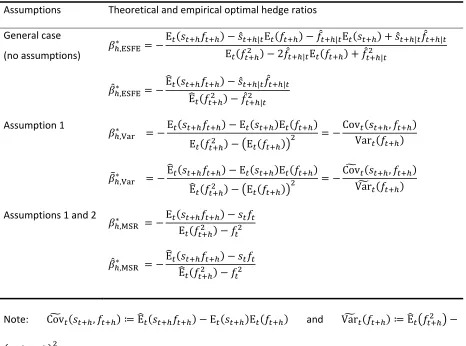
theoretical and empirical optimal hedge ratios in the general case and under additional assumptions
are listed in Table 2.
[Table 2 about here]
4.3 Measures of hedging effectiveness
A natural measure of success (or lack thereof) of hedging is the value of the objective function,
ESFE # * , at the chosen hedge ratio * (e.g. at *?∗,@BA@). It reflects the level of uncertainty over
the future portfolio price in terms of square loss. This study proposes to use ESFE # * as the
theoretical absolute measure of hedging effectiveness. Since ESFE # * is a function of the
7 While *?
,@BA@
∗ is derived in a standard way, by substituting the population quantities with their sample
counterparts, no optimality is claimed for it as an estimator of *∗,@BA@. Finding optimal estimators for *∗,@BA@
16 typically unknown true probability distribution of # , the theoretical measure cannot be applied in
practice, and an empirical counterpart is needed.
Consider sets of ℎ-period-ahead point forecasts of the asset price and the price of the portfolio,
denoted M ̂ | NPO" and M#̂ | NPO", and the corresponding realized prices, Q RPO" and Q# RPO".
Hedging effectiveness can be assessed empirically by mean squared forecast error of the portfolio,
MSFE # , which is the empirical counterpart of ESFE # over the time period = 1, … , U:
MSFE # ≔1T W # − #̂ | P
O"
. (10)
Here, the subscript to the argument of MSFE is +ℎ, indicating the forecast horizon. MSFE # is
the empirical absolute measure of hedging effectiveness under square loss.
Hedging performance can also be gauged in relative terms by comparing the loss under hedging
to the benchmark of no hedging. Let us define the theoretical relative measure of hedging
effectiveness as the relative reduction in expected squared forecast error (RRESFE) when using the
portfolio in comparison with the case of no hedging,
RRESFE # , ≔ESFE ESFE− ESFE # = 1 −ESFE #ESFE . (11)
RRESFE has an upper bound of unity which corresponds to complete absence of uncertainty, or
perfect predictability of the portfolio price and hence perfect hedging performance:
RRESFE # , = 1 ⇔ ESFE # = 0. The measure is unbounded from below. A value
between zero and one suggests that hedging is somewhat effective as it helps reduce the uncertainty
without completely eliminating it: RRESFE # , > 0 ⇔ 0 < ESFE # < ESFE . A
value of zero indicates that the uncertainty over the portfolio price is as great as that of the
unhedged position, and therefore hedging is completely ineffective: RRESFE # , = 0
⇔ ESFE # = ESFE . A value below zero indicates that hedging increases the expected
squared forecast error and is thus detrimental to the goal of uncertainty reduction:
17 ESFE = 0, but that also implies there is no uncertainty in the future price of the original asset
to begin with, rendering hedging irrelevant.
Similarly, let us define the empirical relative measure of hedging effectiveness as the relative
reduction in mean squared forecast error (RRMSFE) when using the portfolio compared to no
hedging,
RRMSFE # , ≔MSFE MSFE− MSFE # = 1 −MSFE #MSFE , (12)
where MSFE ≔ "
Z∑PO" − ̂ | . The bounds and the interpretation of values of
RRMSFE are analogous to those of RRESFE. The theoretical and empirical, absolute and relative
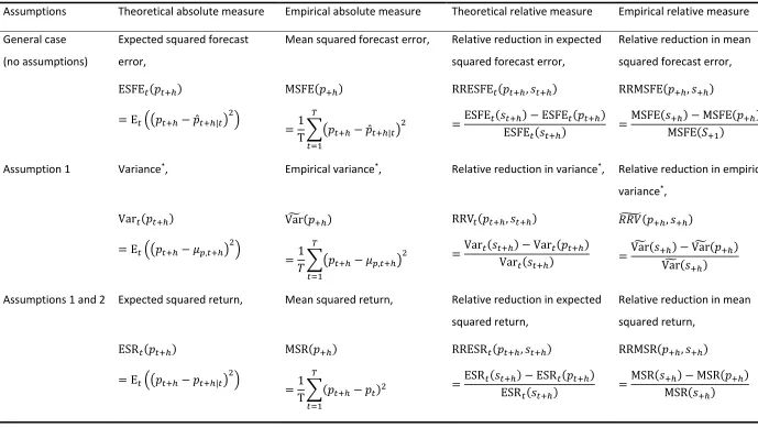
measures of hedging effectiveness in the general case and under additional assumptions are
presented in Table 3.
[Table 3 about here]
4.4 Statistical significance of hedging effectiveness
When measuring hedging effectiveness empirically, estimation errors are unavoidable; hence, the
measured values are imperfect reflections of the true underlying values. Given a measured value,
one may be interested in whether the corresponding true value is different from zero. This is
equivalent to asking whether hedging has any genuine effect on price uncertainty. The null
hypothesis of equally great price uncertainty under hedging versus no hedging can be tested by the
Diebold-Mariano test of equal predictive ability (Diebold, 2015; Diebold & Mariano, 1995; Harvey et
al., 1997). A rejection of the null hypothesis would attest that the effect of hedging is genuine,
whereas a failure to reject would indicate that the evidence is insufficient to conclude so. Testing
whether the hedging effectiveness of two competing strategies is equally great, or assessing the
difference between the true effectiveness and an arbitrary value other than zero are trivial
18
5. Hedging under square loss: two special cases
5.1 Expected values of prices are known
Let us consider a special case of hedging under square loss where the mathematical expectations of
the future prices and # of the original asset and the hedge portfolio Π, respectively, are
assumed to be known at time and are used as point forecasts. (Under square loss, expectations are
optimal point forecasts, therefore it would be suboptimal to use any other forecasts when
expectations are available.)
Assumption 1. The conditional expectations of and # , denoted ]^, ≔ E and
]_, ≔ E # , are known as of time and are used as point forecasts, ̂ | = ]^, and
#̂ | = ]_, .
Corollary 1. Under Assumption 1, the conditional expectation of + , denoted ]`, ≔
E + , is known as of time .
For example, if and - are exchange rates in a liquid currency exchange market or shares of
highly-traded companies, their future prices (at least for a relatively short time period ℎ) can
reasonably be assumed to have a true population mean at their current values, ]^, = and
]`, = +. In other words, a martingale property can be conjectured for and + in short horizons.
Or if is a share of a highly-traded company and there is a 1:10 share split scheduled for some point
in time between and + ℎ, one may assume ]^, = 0.1 ∙ , except perhaps for a rounding error.
Consequently, the mathematical expectation of the future portfolio price for a given hedge ratio * is
known today and is ]_, = ]^, + *]`, .
Under Assumption 1, ̂ | and #̂ | are equal to ]^, and ]_, , respectively, and the
expected squared forecast error of the portfolio price becomes the variance of the portfolio price,
ESFE # = E # − ]_, = Var # according to the definition of variance. Then
the objective function in equation (5) turns into
19 yielding the well-known objective of variance minimization that stems from the classical framework
of Johnson (1960) and Stein (1961). The optimal hedge ratio due to equation (13) is
*∗,abc= −CovVar +, + , (14)
and its sample counterpart is
*?∗,abc= −Cov
d , +
Vard + (15)
(see Appendix for derivations). Here, Covd , + ≔ EH + − ]^, ]`, and
Vard + ≔ EH + − ]`, are estimators of covariance and variance, respectively, which
employ the true first moments ]^, and ]`, rather than their sample counterparts EH and
EH + . The presence of Covd , + and Vard + in the definition of *?∗,abc under
Assumption 1 is in contrast to CovL , + and VarL + in equation (9) for the optimal hedge
ratio in the general case.
Under Assumption 1, the measures of hedging effectiveness collapse as follows. First, the
theoretical absolute measure, i.e. the expected squared forecast error, becomes the variance of the
portfolio price,
ESFE # = Var # , (16)
which is analogous to the change in the objective function from equation (5) to equation (13).
Second, the empirical absolute measure, the mean squared forecast error, becomes the empirical
variance of the portfolio price that employs the true first moment rather than its sample counterpart:
MSFE # = Vard # , (17)
where Vard # ≔"
P∑PO" # − ]_, . An alternative, widespread measure of empirical
variance, VarL # ≔ "
Pe"∑ # − " P∑PO"# P
O" , does not make for a meaningful measure of
portfolio variance (or absolute hedging effectiveness) as it replaces the true expected values with an
estimate of their average, i.e. the mean of realizations Q# RPO", thereby introducing an error.
ill-20 suited measure of hedging effectiveness) unless the true first moments are equal for all between 1
and U: ]_," = ⋯ = ]_,P . In the latter case, VarL # is a valid effectiveness measure, though
inferior to Vard # , which is more efficient. The use of VarL ∙ in place of Vard ∙ in empirical studies
may explain some of the counterintuitive findings in the literature.
Third, the theoreticalrelative measure of hedging effectiveness becomes
RRESFE # , =ESFE ESFE− ESFE
=Var Var − Var #
=: RRV # , ,
(18)
where RRV stands for “relative reduction in variance”, a term and effectiveness measure proposed
by Johnson (1960) and Ederington (1979). RRV is justified as the theoretical relative measure of
hedging effectiveness whenever Assumption 1 holds. Fourth, the empirical relative measure of
hedging effectiveness turns into
RRMSFE # , =MSFE MSFE− MSFE #
=Vard − Vard # Vard
=: RRVg # , .
(19)
where RRVg # , is a plug-in estimator of RRV # , . Just as in the case of the theoretical
relative measure, also here the use of VarL ∙ in place of Vard ∙ is unwarranted following the same
argumentation as above. It may be responsible for the prevalent confusion surrounding the
minimum-variance framework.
5.2 Expected values of prices equal current prices
When the expected future price of an asset is known in advance, it may typically equal the last
observed price as in the examples of the foreign exchange and stock markets in Section 5.1, but
21
Assumption 2. The conditional expectations of and# equal the last observed values of
and #, respectively,]^, = and]_, = # .
Corollary 2. Under Assumption 2, the conditional expectation of + equals the last observed
value of +, ]`, = +.
When the expected price coincides with the last observed price and is used as a point forecast,
the ℎ-step-ahead forecast error is nothing else than the realized price change, or return, from time
to + ℎ. This allows replacing the forecast error with the return in the expressions for the objective
function, the optimal hedge ratio, and the measures of hedging effectiveness. Under Assumptions 1
and 2, the expected squared forecast error of the portfolio price becomes the expected squared
portfolio return, ESFE # = E # − # =: ESR # , leading to the objective function
ESR # * → min(∈;, (20)
which is to minimize the expected squared portfolio return with respect to the hedge ratio *. The
theoretical optimal hedge ratio is implicitly defined as
*∗,@Bh≔ arg min(∈; ESRi # = arg min(∈; E # − # , (21)
which yields the explicit expression
*∗,@Bh= −E E ++ − +− +. (22)
The corresponding empirical optimal hedge ratio is
*?∗,jBh = −EH EH ++ − +− + (23)
(see Appendix for derivations). The theoretical absolute measure of hedging effectiveness is the
expected squared return,
ESFE # = ESR # , (24)
and the empiricalabsolute measure is mean squared return of the portfolio, MSR # ,
MSR # ≔T W #1 − # P
O"
22 The theoretical relative measure of hedging effectiveness becomes the relative reduction in expected
squared return,
RRESR # , ≔ESR ESR− ESR # , (26)
and the corresponding empiricalrelative measure is the relative reduction in mean squared return
when holding the portfolio as compared to holding the original asset alone:
RRMSR # , ≔MSR MSR− MSR # . (27)
Here, MSR =Z"∑PO" − is the mean squared return on the original asset. Of course, it
would generally be wrong to use the measures given in equations (24) to (27) when at least one of
the Assumptions 1 and 2 is violated. The discussion on the inadequacy of VarL in place of Vard in
Section 5.1 applies here, too, with MSR substituting for Vard. That is, the use of VarL instead of MSR
can only be justified when ]_," = ⋯ = ]_,P , but even then VarL is less efficient than MSR as the
estimator for ESR.
5.3 Why minimum-variance framework does not always fail
Even though the classical minimum-variance hedging framework has been demonstrated to fail in
absence of stringent assumptions, it often delivers seemingly sensible results. This section
investigates how this might come about. First, the empirical optimal hedge ratio might nearly or fully
coincide between the classical and the new framework, as the empirical counterpart of the classical
optimal hedge ratio in equation (3) is quite similar to the new empirical optimal hedge ratio in
equation (9). Depending on what estimators are used for the former, the two may even be equal.
Hence, the optimal hedge ratio derived within the classical framework might often be unproblematic.
Second, the classical empirical relative measure of hedging effectiveness, the RRVk ≔
abcLl^lmn eabcLl_lmn
abcLl^lmn , might nearly or fully coincide with the new measure, the RRMSFE. This may
happen when the price forecasts of the original asset and portfolio are their last observed values in
23 given test sample. In such a case, the estimated relative reduction in variance closely matches the
relative reduction in mean squared forecast error. In other words, the reduction in uncertainty as
measured in the classical framework is about the same as in the new framework.
While these observations might be taken as evidence in favour of continued use of the classical
hedging framework, it should be remembered that minimum-variance hedging may or may not fail
depending on the application at hand. On the other hand, the new framework is unconditionally
guaranteed to deliver correct results.
6. Empirical examples
This section exemplifies the main theoretical considerations of Sections 3 to 5 by demonstrating the
performance of the new and the classical hedging frameworks when hedging the spot price risk of
two major commodities, oil (WTI) and natural gas (Henry Hub). It reveals how the estimated
uncertainty and hedging effectiveness differ across the frameworks and shows whether the same or
different hedging strategies are favoured by the relative reduction in mean squared forecast error
versus the relative reduction in variance.8
Hedging the risk of the monthly spot price with a futures contract is considered for the
one-month horizon and for two hedge ratios, the naïve 1:1 and the estimated optimal hedge ratio due to
equation (9). A bivariate time series of spot and futures prices is modelled in 120-month-long rolling
windows. In the oil market, the spot price is predicted with an error-correction model that allows it
to adjust towards the futures price. The futures price of a given contract is treated as a martingale,
hence its forecast equals the last observed value. In the natural gas market, the futures price of the
relevant contract is taken as a point forecast for both spot and futures prices in the next month. The
optimal hedge ratio is obtained from a bivariate GARCH(1,1)-DCC(1,1) model (Bollerslev, 1986; Engle,
2002) applied on in-sample forecast errors of the two price series.
8 Another application of the new framework is available in Bloznelis (2018), who considers hedging the spot
24 The spot price data is obtained from the WIKI Commodities Prices database at Quandl, and the
futures prices are taken from Chicago Mercantile Exchange via Quandl. The oil price data covers May
1983 to August 2017 (412 data points), while the natural gas price data covers May 1990 to August
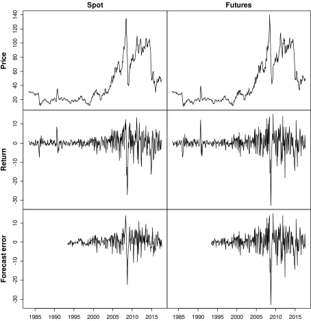
2017 (328 data points). Figures 2 to 5 depict the spot and futures prices of oil and natural gas
together with their returns and forecast errors, alongside the returns and the forecast errors of the
hedge portfolios.
[Figures 2, 3, 4, and 5 around here]
In the case of oil, the forecast errors of spot and portfolio prices are visibly smaller in magnitude
than the respective returns, suggesting that there is a material discrepancy between uncertainty
measured as a function of returns (in the classical framework) versus forecast errors (in the new
framework). This can be seen from the first, third, fourth, and last columns of Table 4 that contains
the hedging results for oil. The variances of the spot and portfolio prices are considerably (up to three
times) higher than the corresponding mean squared forecast errors. Hence, variance and expected
squared forecast error are far from interchangeable, attesting that the former is not an adequate
proxy for the latter. Indeed, variance is an ill-suited measure of uncertainty under square loss,
because not all variability in returns is unpredictable, and the magnitude of returns overestimates
the inherent uncertainty. The exception here is the futures price; the model treats the returns on
futures contracts as entirely unpredictable, which makes them coincide with the forecast errors.
[Table 4 around here]
The last two columns of Table 4 display the readings of the RRV and the RRMSFE, which can be
either similar, as in the case of the 1:1 hedge ratio, or quite different, as in the case of the optimal
hedge ratio. Therefore, the RRV cannot be used in place of the RRMSFE as an innocuous alternative
or an approximation. Moreover, the two measures may also have different subject-matter
implications. E.g. a potential hedger might find a 51% reduction in uncertainty (due to RRV)
25 RRMSFE) might seem large enough to spur her into action. Thus relying on RRV in place of RRMSFE
might make her miss the opportunity to effectively reduce the price uncertainty.
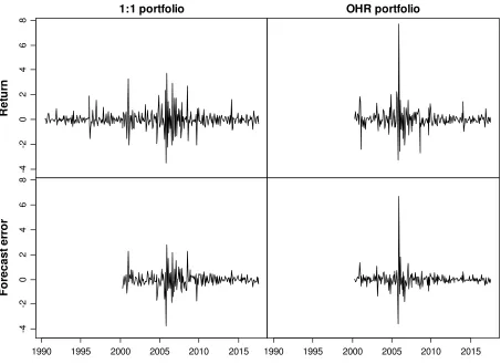
The case of natural gas underscores the qualitative difference in implications of the two
frameworks even more clearly; compare the last two columns in Table 5. While RRV is negative and
hence suggests hedging is detrimental, i.e. it increases uncertainty, RRMSFE is positive and thus
indicates hedging is moderately helpful. The two measures point to opposite directions, and once
again, following the irrelevant measure might lead to suboptimal choices in risk management.
[Table 5 around here]
In summary, real-world hedging applications in major commodity markets highlight pronounced
differences between the classical and the new hedging frameworks. They confirm that the variance
of the portfolio price can be very different from the corresponding expected squared forecast error,
and that RRV and RRMSFE need not be alike. As such, the classical framework of minimum variance
hedging may realistically lead to different implications and hedging decisions than the new
framework of minimum expected squared forecast error. Since hedging is fundamentally concerned
with risk minimization, it is only the latter framework that is adequate for the purpose.
7. Conclusion
Minimum-variance hedging framework has been a highly popular approach to hedging both in the
financial world and in the academic literature starting from the early 1960s. Nearly six decades after
its origins in Johnson (1960) and Stein (1961), it remains the starting point for introducing non-naïve
hedging strategies with futures contracts in finance textbooks (Hull, 2012, p. 57; McDonald, 2013,
p. 114). Despite its continued popularity among practitioners and the extensive academic research
addressing its theoretical as well as applied facets, a key weakness of the minimum-variance hedging
framework has gone unidentified and unexplained so far. It consists of two elements: (1) the fact that
uncertainty over a future price may be better characterized by the probability distribution of its
26 sensible measure of uncertainty, whereas the second moment is. Even though broadly overlooked,
this weakness has created considerable confusion, as the intuitively perceived uncertainty would
repeatedly fail to match the formalized uncertainty estimated in the minimum-variance framework.
While the variance of the hedge portfolio price would be successfully minimized, the perceived
uncertainty (reflected by the magnitude of the expected squared forecast error) would still be
looming large. Also, hedging strategies that incorporate additional information in the price models
would paradoxically yet routinely be found inferior to ones that ignore it.
This work has pinned down and explicitly formulated the previously elusive problem with the
classical minimum-variance hedging framework. It also offers a simple and complete solution to it in
the form of a new hedging framework that generalizes and extends the classical one. Instead of
aiming to minimize the variance of the portfolio price, the actual goal of a hedger might indeed be to
minimize the expected squared forecast error. Once an appropriate objective is adapted, it gives rise
to a new optimal hedge ratio and a new measure of hedging effectiveness. Taken together, the
objective, the ratio, and the effectiveness measure constitute the new framework of hedging under
square loss. This framework applies without restrictions as long as the objective is relevant, and it
contains the minimum-variance framework as a special case, namely, under the assumption that the
true conditional expectations of the future prices of the original asset and the portfolio are known in
advance and are used as point forecasts.
The implications of replacing the classical framework with the new one are substantial. First,
confusion is eliminated as the formalized hedging objective now properly reflects the hedger’s goal.
In turn, measurement of uncertainty is now intuitive and well defined, so that intuitively perceived
and measured effectiveness agree. Second, decisions on the choice of best hedging strategies are
better informed, since hedging strategies that emerge as optimal under the new framework generally
differ from those due to the classical one. Empirical examples from hedging in the oil and natural gas
27 depending on which framework is referred to. Overall, the new framework should thus be of
immediate interest to hedgers and policymakers in commodity and financial markets.
Appropriate measurement of uncertainty introduced in this study is relevant in a much broader
context than hedging alone. Uncertainty underlies significant subfields of finance, economics, and
operations research, among other disciplines. For example, modern portfolio theory, i.e. the
mean-variance framework (Markowitz, 1952), relies on the mean-variance of the portfolio return as representing
the risk. Should variance be replaced by the expected squared forecast error, the theory would need
to be revised. Uncertainty is also a critical element in decision-making problems. Therefore, improved
understanding of uncertainty and the availability of a proper measure thereof can be instrumental in
making better decisions. To conclude, the new measure of uncertainty opens new avenues for
improvement in the context of hedging under square loss, hedging in general, and beyond.
Embracing the new measure and the ensuing hedging framework and examining the broad range of
implications are directions for future research.
8. Acknowledgements
The author is indebted to Ole Gjølberg, Mindaugas Bloznelis, Arnar Mar Buason, Aytac Erdemir, Thilo
Meyer-Brandis, Erik Smith-Meyer, Tom Erik Sønsteng Henriksen, and Andrej Stenšin for their helpful
comments and discussions. Kotryna Bloznelyte has provided excellent editorial suggestions to an
earlier draft. There being no co-authors, the author assumes full responsibility for any omissions and
28
Bibliography
Alexander, C., & Barbosa, A. (2007). Effectiveness of minimum-variance hedging. The Journal of
Portfolio Management, 33(2), 46-59.
Bell, D. E., & Krasker, W. S. (1986). Estimating hedge ratios. Financial Management, 15(2), 34-39.
Bloznelis, D. (2018). Hedging salmon price risk. Aquaculture Economics & Management, 22(2),
168-191.
Bollerslev, T. (1986). Generalized autoregressive conditional heteroskedasticity. Journal of
Econometrics, 31(3), 307-327.
Diebold, F. X. (2015). Comparing predictive accuracy, twenty years later: A personal perspective on
the use and abuse of Diebold–Mariano tests. Journal of Business & Economic Statistics, 33(1),
1-9.
Diebold, F. X. & Mariano, R. S. (1995). Comparing predictive accuracy. Journal of Business & Economic
Statistics, 13(3), 253-263.
Ederington, L. H. (1979). The hedging performance of the new futures markets. The Journal of
Finance, 34(1), 157-170.
Ederington, L. H., & Salas, J. M. (2008). Minimum variance hedging when spot price changes are
partially predictable. Journal of Banking & Finance, 32(5), 654-663.
Engle, R. (2002). Dynamic conditional correlation: A simple class of multivariate generalized
autoregressive conditional heteroskedasticity models. Journal of Business & Economic
Statistics, 20(3), 339-350.
Hardy, C. O., & Lyon, L. S. (1923). The theory of hedging. Journal of Political Economy, 31(2), 276-287.
Harvey, D., Leybourne, S., & Newbold, P. (1997). Testing the equality of prediction mean squared
errors. International Journal of Forecasting, 13(2), 281-291.
Hauser, R. J., Garcia, P., & Tumblin, A. D. (1990). Basis expectations and soybean hedging
29 Hilliard, J. E. (1984). Hedging interest rate risk with futures portfolios under term structure effects.
The Journal of Finance, 39(5), 1547-1569.
Hoffman, G. W. (1931). The Hedging of Grain. The Annals of the American Academy of Political and
Social Science, 155, 7-22.
Hull, J. C. (2012). Options, futures, and other derivatives. London: Pearson Education Limited.
Johnson, L. L. (1960). The theory of hedging and speculation in commodity futures. The Review of
Economic Studies, 27(3), 139-151.
Kahl, K. H. (1983). Determination of the recommended hedging ratio. American Journal of
Agricultural Economics, 65(3), 603-605.
Kaldor, N. (1940). A note on the theory of the forward market. The Review of Economic Studies, 7(3),
196-201.
Lien, D. (2005a). A note on the superiority of the OLS hedge ratio. Journal of Futures Markets, 25(11),
1121-1126.
Lien, D. (2005b). The use and abuse of the hedging effectiveness measure. International Review of
Financial Analysis, 14(2), 277-282.
Lien, D. (2008). A further note on the optimality of the OLS hedge strategy. Journal of Futures
Markets, 28(3), 308-311.
Lindahl, M. (1989). Measuring hedging effectiveness with R2: A note. Journal of Futures Markets,
9(5), 469-475.
Markowitz, H. (1952). Portfolio selection. The Journal of Finance, 7(1), 77-91.
McDonald, R. L. (2013). Derivatives markets. Boston: Pearson Education.
Myers, R. J., & Thompson, S. R. (1989). Generalized optimal hedge ratio estimation. American Journal
of Agricultural Economics, 71(4), 858-868.
Stein, J. L. (1961). The simultaneous determination of spot and futures prices. The American
30 Viswanath, P. V. (1993). Efficient use of information, convergence adjustments, and regression
estimates of hedge ratios. Journal of Futures Markets, 13(1), 43-53.
Working, H. (1953). Futures Trading and Hedging. The American Economic Review, 43(3), 314-343.
Working, H. (1962). New concepts concerning futures markets and prices. The American Economic
31
[image:32.595.66.537.135.344.2]Appendix A: Tables
Table 1 Some measures of uncertainty and their characteristics
Measure (moment of
forecast error distribution)
Value Magnitude
of
uncertainty
Is informative of
the magnitude of
uncertainty
Minimizing the measure
is equivalent to
minimizing uncertainty
First moment, i.e.
mathematical expectation
Close to zero Unknown No No
Far from zero High Yes
First absolute moment Close to zero Low Yes Yes
Far from zero High Yes
Second moment Close to zero Low Yes Yes
Far from zero High Yes
Second central moment, i.e.
variance
Close to zero Unknown No* No*
Far from zero High Yes
32
Table 2 Theoretical and empirical optimal hedge ratios under different assumptions on expected
prices
Assumptions Theoretical and empirical optimal hedge ratios
General case
(no assumptions) * ,@BA@
∗ = −E + − ̂ | E + − +? | E + ̂ | +? | E + − 2+? | E + + +? |
*?∗,@BA@= −EH EH ++ − ̂− +? | +? | |
Assumption 1
*∗,abc = −E + − E E +
E + − E + = −
Cov , + Var +
*o∗,abc = −EH + − E E +
EH + − E + = −
Covd , + Vard +
Assumptions 1 and 2
*∗,jBh = −E E ++ − +− +
*?∗,jBh = −EH EH ++ − +− +
Note: Covd , + ≔ EH + − E E + and Vard + ≔ EH + −
E + are the estimators of covariance and variance, respectively, that employ the true first
moments E of and E + of + rather than their respective sample counterparts
EH and EH + .
Assumption 1. The conditional expectations of and # , denoted ]^, ≔ E and
]_, ≔ E # , are known as of time and are used as point forecasts, ̂ | = ]^, and
#̂ | = ]_, .
Assumption 2. The conditional expectations of and# equal the last observed values of and
Table 3 Measures of hedging effectiveness under different assumptions on expected prices
Assumptions Theoretical absolute measure Empirical absolute measure Theoretical relative measure Empirical relative measure
General case
(no assumptions)
Expected squared forecast
error,
Mean squared forecast error, Relative reduction in expected
squared forecast error,
Relative reduction in mean
squared forecast error,
ESFE #
= E # − #̂ |
MSFE #
=T W #1 − #̂ | P
O"
RRESFE # ,
=ESFE ESFE− ESFE #
RRMSFE # ,
=MSFE MSFE p− MSFE # "
Assumption 1 Variance*, Empirical variance*, Relative reduction in variance*, Relative reduction in empirical
variance*,
Var #
= E # − ]_,
Vard #
=U W #1 − ]_, P
O"
RRV # ,
=Var Var− Var #
qq4g # ,
=Vard Vard− Vard #
Assumptions 1 and 2 Expected squared return, Mean squared return, Relative reduction in expected
squared return,
Relative reduction in mean
squared return,
ESR #
= E # − # |
MSR #
=T W #1 − # P
O"
RRESR # ,
=ESR ESR− ESR #
RRMSR # ,
=MSR MSR− MSR #
Table 4 Results of hedging the monthly spot price of oil (WTI) with oil futures contracts
Effectiveness
measure
Spot Futures Portfolio
1:1
Portfolio
OHR
Relative
reduction 1:1
Relative
reduction OHR
MSFE 13.41 27.11 7.52 3.52 0.44 0.74
Variance 22.44 27.10 13.10 10.89 0.42 0.51
Note: The hedging period is from June 1993 to August 2017. Rolling windows of 120 months are used
for estimating the optimal hedge ratio. Hedging horizon is 1 month ahead. 1:1 denotes the naive 1:1
hedge ratio; OHR denotes the estimated optimal hedge ratio due to equation (9).
Table 5 Results of hedging the monthly spot price of natural gas (Henry Hub) with natural gas
futures contracts
Effectiveness
measure
Spot Futures Portfolio
1:1
Portfolio
OHR
Relative
reduction 1:1
Relative
reduction OHR
MSFE 0.51 0.91 0.42 0.45 0.18 0.12
Variance 0.70 0.91 0.71 0.75 -0.02 -0.08
Note: The hedging period is from June 2000 to August 2017. Rolling windows of 120 months are used
for estimating the optimal hedge ratio. Hedging horizon is 1 month ahead. 1:1 denotes the naive 1:1
[image:35.595.63.530.409.491.2]35
[image:36.595.67.518.157.687.2]Appendix B: Figures
Figure 1 Illustrations of measures of uncertainty for different distributions of forecast error
a) Low uncertainty b) High uncertainty
Light-tailed distribution, symmetric around zero. Heavy-tailed distribution, symmetric around zero.
E | = 0, E | small, E | = 0 (!), E | large,
E | small, Var | small E | large, Var | large
c) High uncertainty d) High uncertainty
Light-tailed distr., symmetric around a large value. Distribution with a unit mass at a large value.
E | large, E | large E | large, E | large,
E | large, Var | small (!) E | large, Var | = 0 (!)
Note: | denotes the forecast error resulting from a forecast made at time for a target
variable at time + ℎ. E ∙ and Var ∙ are the mathematical expectation and variance,
respectively, conditional on the information available at time . |∙| is the absolute value operator.
-4 -2 0 2 4
0 .0 0 .2 0 .4 0 .6 0 .8 1 .0
-4 -2 0 2 4
0 .0 0 .2 0 .4 0 .6 0 .8 1 .0
4 6 8 10 12
0 .0 0 .2 0 .4 0 .6 0 .8 1 .0
-4 -2 0 2 4
36
Figure 2 Spot and futures prices, returns, and forecast errors of oil (WTI)
Note: Monthly data from May 1983 to August 2017 (412 data points). Return denotes price change.
2 0 4 0 6 0 8 0 1 0 0 1 2 0 1 4 0 Spot P ri c e Futures -3 0 -2 0 -1 0 0 1 0 R e tu rn
1985 1990 1995 2000 2005 2010 2015
-3 0 -2 0 -1 0 0 1 0 F o re c a s t e rr o r
37
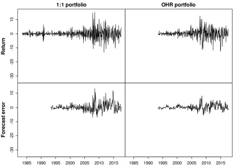
Figure 3 Hedge portfolio returns and forecast errors of oil (WTI)
Note: Monthly data from May 1983 to August 2017 (412 data points). Return denotes price change;
(1:1) denotes naïve 1:1 hedge ratio; (OHR) denotes estimated optimal hedge ratio due to
equation (9).
-3
0
-2
0
-1
0
0
1
0
1:1 portfolio
R
e
tu
rn
OHR portfolio
1985 1990 1995 2000 2005 2010 2015
-3
0
-2
0
-1
0
0
1
0
F
o
re
c
a
s
t
e
rr
o
r
38
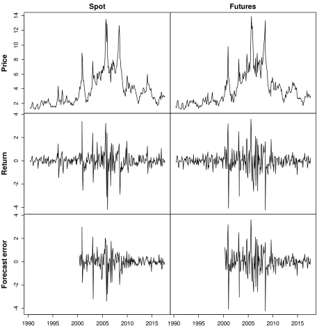
Figure 4 Spot and futures prices, returns, and forecast errors of natural gas (Henry Hub)
Note: Monthly data from May 1990 to August 2017 (328 data points). Return denotes price change.
2 4 6 8 1 0 1 2 1 4 Spot P ri c e Futures -4 -2 0 2 4 R e tu rn
1990 1995 2000 2005 2010 2015
-4 -2 0 2 4 F o re c a s t e rr o r