Riemannian Optimization for Skip Gram Negative Sampling

(1)

Proceedings of the 55th Annual Meeting of the Association for Computational Linguistics, pages 2028–2036 Vancouver, Canada, July 30 - August 4, 2017. c2017 Association for Computational Linguistics

Riemannian Optimization for Skip-Gram Negative Sampling

Alexander Fonarev1,2,4,*_,_{Oleksii Hrinchuk}1,2,3,*_,

Gleb Gusev2,3_,_{Pavel Serdyukov}2_{, and}_{Ivan Oseledets}1,5 1_{Skolkovo Institute of Science and Technology, Moscow, Russia}

2_{Yandex LLC, Moscow, Russia}

3_{Moscow Institute of Physics and Technology, Moscow, Russia} 4_{SBDA Group, Dublin, Ireland}

5_{Institute of Numerical Mathematics, Russian Academy of Sciences, Moscow, Russia}

Abstract

Skip-Gram Negative Sampling (SGNS) word embedding model, well known by its implementation in “word2vec” software, is usually optimized by stochastic gradi-ent descgradi-ent. However, the optimization of SGNS objective can be viewed as a prob-lem of searching for a good matrix with the low-rank constraint. The most stan-dard way to solve this type of problems is to apply Riemannian optimization frame-work to optimize the SGNS objective over the manifold of required low-rank matri-ces. In this paper, we propose an algo-rithm that optimizes SGNS objective us-ing Riemannian optimization and demon-strates its superiority over popular com-petitors, such as the original method to train SGNS and SVD over SPPMI matrix. 1 Introduction

In this paper, we consider the problem of embed-ding words into a low-dimensional space in order to measure the semantic similarity between them. As an example, how to find whether the word “table” is semantically more similar to the word “stool” than to the word “sky”? That is achieved by constructing a low-dimensional vector repre-sentation for each word and measuring similarity between the words as the similarity between the corresponding vectors.

One of the most popular word embedding mod-els (Mikolov et al.,2013) is a discriminative neu-ral network that optimizes Skip-Gram Negative Sampling (SGNS) objective (see Equation3). It aims at predicting whether two words can be found close to each other within a text. As shown in Sec-tion 2, the process of word embeddings training

∗_{The first two authors contributed equally to this work}

using SGNS can be divided into two general steps with clear objectives:

Step 1. Search for a low-rank matrixX that

pro-vides a good SGNS objective value; Step 2. Search for a good low-rank representation

X =W C>in terms of linguistic metrics, whereW is a matrix of word embeddings

andCis a matrix of so-called context

em-beddings.

Unfortunately, most previous approaches mixed these two steps into a single one, what entails a not completely correct formulation of the optimization problem. For example, popular approaches to train embeddings (including the original “word2vec” implementation) do not take into account that the objective from Step 1 depends only on the prod-uctX = W C>: instead of straightforward

com-puting of the derivative w.r.t. X, these methods are explicitly based on the derivatives w.r.t. W

andC, what complicates the optimization

proce-dure. Moreover, such approaches do not take into account that parametrizationW C>of matrixXis

non-unique and Step 2 is required. Indeed, for any invertible matrixS, we have

X=W1C1>=W1SS−1C1>=W2C2>,

therefore, solutionsW1C1>andW2C2>are equally

good in terms of the SGNS objective but entail different cosine similarities between embeddings and, as a result, different performance in terms of linguistic metrics (see Section4.2for details).

A successful attempt to follow the above de-scribed steps, which outperforms the original SGNS optimization approach in terms of various linguistic tasks, was proposed in (Levy and Gold-berg,2014). In order to obtain a low-rank matrix

Xon Step 1, the method reduces the

(2)

tion (SPPMI) matrix via Singular Value Decom-position (SVD). On Step 2, it computes embed-dingsW andCvia a simple formula that depends

on the factors obtained by SVD. However, this method has one important limitation: SVD pro-vides a solution to a surrogate optimization prlem, which has no direct relation to the SGNS ob-jective. In fact, SVD minimizes the Mean Squared Error (MSE) betweenXand SPPMI matrix, what

does not lead to minimization of SGNS objec-tive in general (see Section 6.1 and Section 4.2 in (Levy and Goldberg,2014) for details).

These issues bring us to the main idea of our paper: while keeping the low-rank matrix search setup on Step 1, optimize the original SGNS objective directly. This leads to an opti-mization problem over matrix X with the

low-rank constraint, which is often (Mishra et al., 2014) solved by applying Riemannian optimiza-tionframework (Udriste,1994). In our paper, we use the projector-splitting algorithm (Lubich and Oseledets,2014), which is easy to implement and has low computational complexity. Of course, Step 2 may be improved as well, but we regard this as a direction of future work.

As a result, our approach achieves the signif-icant improvement in terms of SGNS optimiza-tion on Step 1 and, moreover, the improvement on Step 1 entails the improvement on Step 2 in terms of linguistic metrics. That is why, the proposed two-step decomposition of the problem makes sense, what, most importantly, opens the way to applying even more advanced approaches based on it (e.g., more advanced Riemannian opti-mization techniques for Step 1 or a more sophisti-cated treatment of Step 2).

To summarize, the main contributions of our pa-per are:

• We reformulated the problem of SGNS word embedding learning as a two-step procedure with clear objectives;

• For Step 1, we developed an algorithm based on Riemannian optimization framework that optimizes SGNS objective over low-rank ma-trixXdirectly;

• Our algorithm outperforms state-of-the-art competitors in terms of SGNS objective and the semantic similarity linguistic met-ric (Levy and Goldberg,2014;Mikolov et al., 2013;Schnabel et al.,2015).

2 Problem Setting

2.1 Skip-Gram Negative Sampling

In this paper, we consider the Skip-Gram Negative Sampling (SGNS) word embedding model (Mikolov et al., 2013), which is a prob-abilistic discriminative model. Assume we have a text corpus given as a sequence of words

w1, . . . , wn, wherenmay be larger than1012and wi∈VW belongs to a vocabulary of wordsVW. A

contextc_∈ VC of the wordwiis a word from set {wi−L, ..., wi−1, wi+1, ..., wi+L} for some fixed

window sizeL. Letw,c ∈ Rd_{be the}_word

em-beddings of word w and context c, respectively.

Assume they are specified by the following map-pings:

W :VW →Rd, C:VC →Rd.

The ultimate goal of SGNS word embedding train-ing is to fit good mapptrain-ingsW andC.

Let D be a multiset of all word-context pairs

observed in the corpus. In the SGNS model, the probability that word-context pair (w, c) is ob-served in the corpus is modeled as a following dsitribution:

P(#(w, c)₆= 0_|w, c) =

=σ(hw,ci) = 1

1 + exp(_−hw,c_i), (1) where #(w, c) is the number of times the pair (w, c) appears in D andhx,yi is the scalar product of vectorsxandy. Numberdis a

hyper-parameter that adjusts the flexibility of the model. It usually takes values from tens to hundreds.

In order to collect a training set, we take all pairs (w, c) from D as positive examples and k

randomly generated pairs(w, c)as negative ones. The number of times the wordwand the contextc

appear inDcan be computed as

#(w) = X

c∈Vc

#(w, c),

#(c) = X

w∈Vw

#(w, c)

accordingly. Then negative examples are gener-ated from the distribution defined by#(c) coun-ters:

PD(c) =

#(c)

(3)

In this way, we have a model maximizing the following logarithmic likelihood objective for all word-context pairs(w, c):

lwc = #(w, c)(logσ(hw,ci)+

+k·Ec0_∼_P_Dlogσ(−hw,c0i)). (2)

In order to maximize the objective over all obser-vations for each pair (w, c), we arrive at the

fol-lowing SGNS optimization problem over all pos-sible mappingsWandC:

l= X

w∈VW

X

c∈VC

(#(w, c)(logσ(hw,ci)+

+k_·Ec0_∼PDlogσ(−hw,c

0_i₎₎₎_→_max W,C .

(3)

Usually, this optimization is done via the stochas-tic gradient descent procedure that is performed during passing through the corpus (Mikolov et al., 2013;Rong,2014).

2.2 Optimization over Low-Rank Matrices Relying on the prospect proposed in (Levy and Goldberg,2014), let us show that the optimization problem given by (3) can be considered as a prob-lem of searching for a matrix that maximizes a certain objective function and has the rank-d

con-straint (Step 1 in the scheme described in Sec-tion1).

2.2.1 SGNS Loss Function

As shown in (Levy and Goldberg, 2014), the logarithmic likelihood (3) can be represented as the sum of lw,c(w,c) over all pairs (w, c),

wherelw,c(w,c)has the following form:

lw,c(w,c) = #(w, c) logσ(hw,ci)+

+k#(w)#(c)

|D| logσ(−hw,ci).

(4)

A crucial observation is that this loss function de-pends only on the scalar producthw,cibut not on embeddingswandcseparately:

lw,c(w,c) =fw,c(xw,c),

where

fw,c(xw,c) =aw,clogσ(xw,c)+bw,clogσ(−xw,c),

andxw,cis the scalar producthw,ci, and aw,c = #(w, c), bw,c=k

#(w)#(c)

|D_|

are constants.

2.2.2 Matrix Notation

Denote|VW|asnand|VC|asm. LetW ∈Rn×d

andC ∈Rm×d_{be matrices, where each row}_w_∈

Rd_{of matrix}_W _{is the word embedding of the}

cor-responding wordwand each rowc _∈ _Rd_of

ma-trixCis the context embedding of the

correspond-ing contextc. Then the elements of the product of

these matrices

X=W C>

are the scalar productsxw,cof all pairs(w, c): X = (xw,c), w∈VW, c∈VC.

Note that this matrix has rankd, becauseXequals

to the product of two matrices with sizes(n×d) and(d_×m). Now we can write SGNS objective

given by (3) as a function ofX: F(X) = X

w∈VW

X

c∈VC

fw,c(xw,c), F :Rn×m →R.

(5) This arrives us at the following proposition: Proposition 1 SGNS optimization problem given by (3) can be rewritten in the following con-strained form:

maximize

X∈Rn×m F(X),

subject to X_{∈ M}d,

(6)

where Md is the manifold (Udriste, 1994) of all

matrices inRn×m_{with rank}_d_:

Md={X∈Rn×m :rank(X) =d}.

The key idea of this paper is to solve the opti-mization problem given by (6) via the framework of Riemannian optimization, which we introduce in Section3.

Important to note that this prospect does not suppose the optimization over parameters W

and C directly. This entails the optimization in

the space with((n+m−d)·d)degrees of free-dom (Mukherjee et al.,2015) instead of((n+m)· d), what simplifies the optimization process (see

Section5for the experimental results). 2.3 Computing Embeddings from a

Low-Rank Solution

OnceX is found, we need to recover W andC

such that X = W C> (Step 2 in the scheme

(4)

have a unique solution, since if(W, C)satisfy this equation, thenW S−1 andCS>satisfy it as well

for any non-singular matrixS. Moreover, different

solutions may achieve different values of the lin-guistic metrics (see Section4.2for details). While our paper focuses on Step 1, we use, for Step 2, a heuristic approach that was proposed in (Levy et al.,2015) and it shows good results in practice. We compute SVD ofXin the form

X=UΣV>,

whereU andV have orthonormal columns, andΣ is the diagonal matrix, and use

W =U√Σ, C=V√Σ as matrices of embeddings.

A simple justification of this solution is the fol-lowing: we need to map words into vectors in a way that similar words would have similar embed-dings in terms of cosine similarities:

cos(w1,w2) = h

w1,w2i

kw1k · kw2k .

It is reasonable to assume that two words are sim-ilar, if they share contexts. Therefore, we can esti-mate the similarity of two wordsw1,w2as

s(w1, w2) =

X

c∈VC

xw1,c·xw2,c,

what is the element of the matrixXX> with

in-dices(w1, w2). Note that

XX>=UΣV>VΣU>=UΣ2U>.

If we choose W = UΣ, we exactly

ob-tain hw1,w2i = s(w1, w2), since W W> = XX> in this case. That is, the cosine

similar-ity of the embeddings w1,w2 coincides with the

intuitive similarity s(w1, w2). However, scaling

by √Σ instead of Σ was shown in (Levy et al., 2015) to be a better solution in experiments.

3 Proposed Method

3.1 Riemannian Optimization 3.1.1 General Scheme

The main idea of Riemannian optimiza-tion (Udriste, 1994) is to consider (6) as a constrained optimization problem. Assume we have an approximated solution Xi on a current

step of the optimization process, where i is the step number. In order to improveXi, the next step

of the standard gradient ascent outputs the point

Xi+∇F(Xi),

where ∇F(Xi) is the gradient of objective F at

the point Xi. Note that the gradient ∇F(Xi)

can be naturally considered as a matrix inRn×m_.

Point Xi + ∇F(Xi) leaves the manifold Md,

because its rank is generally greater than d.

That is why Riemannian optimization methods map point Xi +∇F(Xi) back to manifoldMd.

The standard Riemannian gradient method first projects the gradient step onto the tangent space at the current pointXi and thenretractsit back to

the manifold:

Xi+1 =R(PTM(Xi+∇F(Xi))),

whereRis theretractionoperator, andP_T_M is the

projection onto the tangent space.

Although the optimization problem is non-convex, Riemannian optimization methods show good performance on it. Theoretical properties and convergence guarantees of such methods are discussed in (Wei et al.,2016) more thoroughly. 3.1.2 Projector-Splitting Algorithm

In our paper, we use a simplified version of such approach that retracts pointXi+∇F(Xi)directly to the manifold and does not require projection onto the tangent space P_T_M as illustrated in

Fig-ure1:

Xi+1 =R(Xi+∇F(Xi)).

Intuitively, retractorRfinds a rank-dmatrix on the manifoldMdthat is similar to high-rank

ma-trix Xi +∇F(Xi) in terms of Frobenius norm.

How can we do it? The most straightforward way to reduce the rank ofXi+∇F(Xi)is to perform the SVD, which keepsdlargest singular values of

it:

1:Ui+1, Si+1, Vi>+1←SVD(Xi+∇F(Xi)),

2:Xi+1 ←Ui+1Si+1Vi>+1.

(5)

Fine-tuning word embeddings

xxxxx xxxxx

xxxxx xxxx xxxxxxxx xxx xxxxx xxxxxxxxx

ABSTRACT

Blah-blah

Keywords

word embeddings, SGNS, word2vec, GLOVE

1. INTRODUCTION

sdfdsf

2. CONCLUSIONS

3. RELATED WORK

Mikolov main [?] Levi main [?]

rFi

Xi=UiSiViT

Xi+1=Ui+1Si+1ViT+1

retraction

4. CONCLUSIONS

Permission to make digital or hard copies of all or part of this work for personal or classroom use is granted without fee provided that copies are not made or distributed for profit or commercial advantage and that copies bear this notice and the full citation on the first page. To copy otherwise, to republish, to post on servers or to redistribute to lists, requires prior specific permission and/or a fee.

WOODSTOCK’97 El Paso, Texas USA

Copyright 20XX ACM X-XXXXX-XX-X/XX/XX ...$15.00.

Fine-tuning word embeddings

xxxxx xxxxx

ABSTRACT

Blah-blah

Keywords

1. INTRODUCTION

sdfdsf

2. CONCLUSIONS

3. RELATED WORK

rFi

Xi=UiSiViT

Xi+1=Ui+1Si+1ViT+1

retraction

Md

4. CONCLUSIONS

Fine-tuning word embeddings

xxxxx xxxxx

ABSTRACT

Blah-blah

Keywords

1. INTRODUCTION

sdfdsf

2. CONCLUSIONS

3. RELATED WORK

rF(Xi)

Xi+rF(Xi)

Xi=UiSiViT

Xi

Xi+1

Xi+1=Ui+1Si+1ViT+1

retraction

Md

4. CONCLUSIONS

Fine-tuning word embeddings

xxxxx xxxxx

ABSTRACT

Blah-blah

Keywords

1. INTRODUCTION

sdfdsf

2. CONCLUSIONS

3. RELATED WORK

rF(Xi)

Xi+rF(Xi)

Xi=UiSiViT

Xi

Xi+1

Xi+1=Ui+1Si+1ViT+1

retraction

Md

4. CONCLUSIONS

Fine-tuning word embeddings

xxxxx xxxxx

ABSTRACT

Blah-blah

Keywords

1. INTRODUCTION

sdfdsf

2. CONCLUSIONS

3. RELATED WORK

rF(Xi)

Xi+rF(Xi)

Xi=UiSiViT

Xi

Xi+1

Xi+1=Ui+1Si+1ViT+1

retraction

Md

4. CONCLUSIONS

Fine-tuning word embeddings

xxxxx xxxxx

ABSTRACT

Blah-blah

Keywords

1. INTRODUCTION

sdfdsf

2. CONCLUSIONS

3. RELATED WORK

rF(Xi)

Xi+rF(Xi)

Xi=UiSiViT

Xi

Xi+1

Xi+1=Ui+1Si+1ViT+1

retraction

Md

4. CONCLUSIONS

Figure 1: Geometric interpretation of one step of projector-splitting optimization procedure: the gradient step an the retraction of the high-rank ma-trixXi+∇F(Xi)to the manifold of low-rank

ma-trices Md.

also quite intuitive: instead of computing the full SVD of Xi +∇F(Xi) according to the

gradi-ent projection method, we use just one step of the block power numerical method (Bentbib and Kan-ber,2015) which computes the SVD, what reduces the computational complexity.

Let us keep the current point in the following factorized form:

Xi =UiSiV_i>, (8)

where matricesUi∈Rn×dandVi ∈Rm×dhaved

orthonormal columns andSi ∈ Rd×d. Then we

need to perform two QR-decompositions to retract pointXi+∇F(Xi)back to the manifold:

1:Ui+1, Si+1←QR((Xi+∇F(Xi))Vi),

2:Vi+1, S>i+1←QR

(Xi+∇F(Xi))>Ui+1

,

3:Xi+1 ←Ui+1Si+1Vi>+1.

In this way, we always keep the solutionXi+1 = Ui+1Si+1Vi>+1 on the manifold Md and in the

form (8).

What is important, we only need to com-pute ∇F(Xi), so the gradients with respect to U, S andV are never computed explicitly, thus

avoiding the subtle case whereSis close to

singu-lar (so-called singusingu-lar (critical) point on the man-ifold). Indeed, the gradient with respect to U

(while keeping the orthogonality constraints) can be written (Koch and Lubich,2007) as:

∂F

∂U =

∂F ∂XV S

−1_,

which means that the gradient will be large ifSis close to singular. The projector-splitting scheme is free from this problem.

3.2 Algorithm

In case of SGNS objective given by (5), an element of gradient∇F has the form:

(_∇F(X))w,c=

∂fw,c(xw,c)

∂xw,c =

= #(w, c)·σ(−xw,c)−k#(w)#(c)

|D_| ·σ(xw,c).

To make the method more flexible in terms of con-vergence properties, we additionally use λ ∈ R, which is a step size parameter. In this case, re-tractorRreturnsXi+λ∇F(Xi)instead ofXi+ ∇F(Xi)onto the manifold.

The whole optimization procedure is summa-rized in Algorithm1.

4 Experimental Setup 4.1 Training Models

We compare our method (“RO-SGNS” in the ta-bles) performance to two baselines: SGNS embed-dings optimized via Stochastic Gradient Descent, implemented in the original “word2vec”, (“SGD-SGNS” in the tables) (Mikolov et al., 2013) and embeddings obtained by SVD over SPPMI ma-trix (“SVD-SPPMI” in the tables) (Levy and Gold-berg,2014). We have also experimented with the blockwise alternating optimization over factors W and C, but the results are almost the same to SGD results, that is why we do not to include them into the paper. The source code of our experiments is available online1_.

The models were trained on English Wikipedia “enwik9” corpus2_{, which was previously used in} most papers on this topic. Like in previous stud-ies, we counted only the words which occur more than 200 times in the training corpus (Levy and Goldberg, 2014;Mikolov et al., 2013). As a re-sult, we obtained a vocabulary of 24292 unique tokens (set of wordsVW and set of contexts VC

are equal). The size of the context window was set to5 for all experiments, as it was done in (Levy and Goldberg, 2014; Mikolov et al., 2013). We conduct three series of experiments: for dimen-sionalityd= 100,d= 200, andd= 500.

(6)

Algorithm 1Riemannian Optimization for SGNS

Require: Dimentionalityd, initializationW0 and C0, step size λ, gradient function ∇F : Rn×m →

Rn×m_{, number of iterations}_K

Ensure: FactorW _∈_Rn×d

1: X0 ←W0C0> # get an initial point at the manifold 2: U0, S0, V0>←SVD(X0) # compute the first point satisfying the low-rank constraint 3: fori_←1, . . . , Kdo

4: Ui, Si←QR((Xi₋1+λ∇F(Xi−1))Vi−1) # perform one step of the block power method 5: Vi, Si>←QR (Xi−1+λ∇F(Xi−1))>Ui

6: Xi←UiSiVi> # update the point at the manifold 7: end for

8: U,Σ, V>_←SVD(XK)

9: W _←U√Σ # compute word embeddings

10: return W

Optimization step size is chosen to be small enough to avoid huge gradient values. However, thorough choice of λdoes not result in a

signifi-cant difference in performance (this parameter was tuned on the training data only, the exact values used in experiments are reported below).

4.2 Evaluation

We evaluate word embeddings via the word simi-larity task. We use the following popular datasets for this purpose: “wordsim-353” ((Finkelstein et al.,2001); 3 datasets), “simlex-999” (Hill et al., 2016) and “men” (Bruni et al., 2014). Original “wordsim-353” dataset is a mixture of the word pairs for both word similarity and word related-ness tasks. This dataset was split (Agirre et al., 2009) into two intersecting parts: “wordsim-sim” sim” in the tables) and “wordsim-rel” (“ws-rel” in the tables) to separate the words from dif-ferent tasks. In our experiments, we use both of them on a par with the full version of “wordsim-353” (“ws-full” in the tables). Each dataset con-tains word pairs together with assessor-assigned similarity scores for each pair. As a quality mea-sure, we use Spearman’s correlation between these human ratings and cosine similarities for each pair. We call this quality metriclinguisticin our paper. 5 Results of Experiments

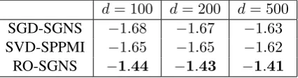
First of all, we compare the value of SGNS objec-tive obtained by the methods. The comparison is demonstrated in Table1.

We see that SGD-SGNS and SVD-SPPMI methods provide quite similar results, however, the proposed method obtains significantly better

[image:6.595.310.523.276.332.2]

d= 100 d= 200 d= 500 SGD-SGNS −1.68 ₋1.67 ₋1.63 SVD-SPPMI −1.65 −1.65 −1.62 RO-SGNS −1.44 ₋1.43 ₋1.41

Table 1: Comparison of SGNS values (multiplied by10−9) obtained by the models. Larger is better.

SGNS values, what proves the feasibility of us-ing Riemannian optimization framework in SGNS optimization problem. It is interesting to note that SVD-SPPMI method, which does not opti-mize SGNS objective directly, obtains better re-sults than SGD-SGNS method, which aims at opti-mizing SGNS. This fact additionally confirms the idea described in Section 2.2.2 that the indepen-dent optimization over parametersW andC may

decrease the performance.

However, the target performance measure of embedding models is the correlation between se-mantic similarity and human assessment (Sec-tion 4.2). Table2presents the comparison of the methods in terms of it. We see that our method outperforms the competitors on all datasets except for “men” dataset where it obtains slightly worse results. Moreover, it is important that the higher dimension entails higher performance gain of our method in comparison to the competitors.

(7)

Dim. d Algorithm ws-sim ws-rel ws-full simlex men d= 100

SGD-SGNS 0.719 0.570 0.662 0.288 0.645 SVD-SPPMI 0.722 0.585 0.669 0.317 0.686 RO-SGNS 0.729 0.597 0.677 0.322 0.683

d= 200

d= 500

[image:7.595.137.461.62.201.2]

Table 2: Comparison of the methods in terms of the semantic similarity task. Each entry represents the Spearman’s correlation between predicted similarities and the manually assessed ones.

five he main

SVD-SPPMI RO-SGNS SVD-SPPMI RO-SGNS SVD-SPPMI RO-SGNS

[image:7.595.82.509.244.322.2]

Neighbors Dist. Neighbors Dist. Neighbors Dist. Neighbors Dist. Neighbors Dist. Neighbors Dist. lb 0.748 four 0.999 she 0.918 when 0.904 major 0.631 major 0.689 kg 0.731 three 0.999 was 0.797 had 0.903 busiest 0.621 important 0.661 mm 0.670 six 0.997 promptly 0.742 was 0.901 principal 0.607 line 0.631 mk 0.651 seven 0.997 having 0.731 who 0.892 nearest 0.607 external 0.624 lbf 0.650 eight 0.996 dumbledore 0.731 she 0.884 connecting 0.591 principal 0.618 per 0.644 and 0.985 him 0.730 by 0.880 linking 0.588 primary 0.612

Table 3: Examples of the semantic neighbors obtained for words “five”, “he” and “main”.

usa

SGD-SGNS SVD-SPPMI RO-SGNS

Neighbors Dist. Neighbors Dist. Neighbors Dist. akron 0.536 wisconsin 0.700 georgia 0.707 midwest 0.535 delaware 0.693 delaware 0.706 burbank 0.534 ohio 0.691 maryland 0.705

nevada 0.534 northeast 0.690 illinois 0.704

arizona 0.533 cities 0.688 madison 0.703

uk 0.532 southwest 0.684 arkansas 0.699 youngstown 0.532 places 0.684 dakota 0.690

utah 0.530 counties 0.681 tennessee 0.689 milwaukee 0.530 maryland 0.680 northeast 0.687 headquartered 0.527 dakota 0.674 nebraska 0.686

Table 4: Examples of the semantic neighbors from11th to20th obtained for the word “usa” by all three methods. Top-10neighbors for all three methods are exact names of states.

source word. First of all, we notice that our model produces much better neighbors of the words de-scribing digits or numbers (see word “five” as an example). Similar situation happens for many other words, e.g. in case of “main” — the nearest neighbors contain 4 similar words for our model instead of 2 in case of SVD-SPPMI. The neigh-bourhood of “he” contains less semantically sim-ilar words in case of our model. However, it fil-ters out irrelevant words, such as “promptly” and “dumbledore”.

Table4contains the nearest words to the word “usa” from 11th to 20th. We marked names of USA states bold and did not represent top-10 near-est words as they are exactly names of states for all three models. Some non-bold words are ar-guably relevant as they present large USA cities

(“akron”, “burbank”, “madison”) or geographi-cal regions of several states (“midwest”, “north-east”, “southwest”), but there are also some com-pletely irrelevant words (“uk”, “cities”, “places”) presented by first two models.

Our experiments show that the optimal number of iterationsK in the optimization procedure and

step size λ depend on the particular value of d.

Ford = 100, we haveK = 7, λ = 5_·10−5_{, for} d= 200, we haveK = 8, λ = 5·10−5, and for

d= 500, we haveK = 2, λ= 10−4. Moreover, the best results were obtained when SVD-SPPMI embeddings were used as an initialization of Rie-mannian optimization process.

Figure2illustrates how the correlation between semantic similarity and human assessment scores changes through iterations of our method. Optimal value ofK is the same for both whole testing set

and its 10-fold subsets chosen for cross-validation. The idea to stop optimization procedure on some iteration is also discussed in (Lai et al.,2015).

Training of the same dimensional models (d= 500) on English Wikipedia corpus using

[image:7.595.66.290.361.466.2]

(8)

0 5 10 15 20 25

iterations

0.692 0.694 0.696 0.698 0.700 0.702 0.704 0.706

0.708 wordsim-353

0 5 10 15 20 25

iterations

0.346 0.347 0.348 0.349 0.350 0.351 0.352 0.353

0.354 simlex-999

0 5 10 15 20 25

iterations

0.696 0.698 0.700 0.702 0.704 0.706 0.708

[image:8.595.86.533.66.168.2]

0.710 men

Figure 2: Illustration of why it is important to choose the optimal iteration and stop optimization proce-dure after it. The graphs show semantic similarity metric in dependence on the iteration of optimization procedure. The embeddings obtained by SVD-SPPMI method were used as initialization. Parameters:

d= 200,λ= 5_·10−5. 6 Related Work 6.1 Word Embeddings

Skip-Gram Negative Sampling was introduced in (Mikolov et al.,2013). The “negative sampling” approach is thoroughly described in (Goldberg and Levy,2014), and the learning method is explained in (Rong, 2014). There are several open-source implementations of SGNS neural network, which is widely known as “word2vec”.12

As shown in Section 2.2, Skip-Gram Negative Sampling optimization can be reformulated as a problem of searching for a low-rank matrix. In or-der to be able to use out-of-the-box SVD for this task, the authors of (Levy and Goldberg, 2014) used the surrogate version of SGNS as the objec-tive function. There are two general assumptions made in their algorithm that distinguish it from the SGNS optimization:

1. SVD optimizes Mean Squared Error (MSE) objective instead of SGNS loss function. 2. In order to avoid infinite elements in SPMI

matrix, it is transformed in ad-hoc manner (SPPMI matrix) before applying SVD. This makes the objective not interpretable in terms of the original task (3). As mentioned in (Levy and Goldberg,2014), SGNS objective weighs dif-ferent (w, c) pairs differently, unlike the SVD, which works with the same weight for all pairs and may entail the performance fall. The compre-hensive explanation of the relation between SGNS and SVD-SPPMI methods is provided in (Keerthi et al.,2015). (Lai et al., 2015;Levy et al.,2015)

1_{Original Google word2vec:} _{https://code.}

google.com/archive/p/word2vec/

2_{Gensim word2vec:} _{https://radimrehurek.}

com/gensim/models/word2vec.html

give a good overview of highly practical methods to improve these word embedding models. 6.2 Riemannian Optimization

An introduction to optimization over Riemannian manifolds can be found in (Udriste, 1994). The overview of retractions of high rank matrices to low-rank manifolds is provided in (Absil and Os-eledets, 2015). The projector-splitting algorithm was introduced in (Lubich and Oseledets, 2014), and also was mentioned in (Absil and Oseledets, 2015) as “Lie-Trotter retraction”.

Riemannian optimization is succesfully applied to various data science problems: for example, matrix completion (Vandereycken, 2013), large-scale recommender systems (Tan et al.,2014), and tensor completion (Kressner et al.,2014).

7 Conclusions

In our paper, we proposed the general two-step scheme of training SGNS word embedding model and introduced the algorithm that performs the search of a solution in the low-rank form via Riemannian optimization framework. We also demonstrated the superiority of our method by providing experimental comparison to existing state-of-the-art approaches.

Possible direction of future work is to apply more advanced optimization techniques to the Step 1 of the scheme proposed in Section1and to explore the Step 2 — obtaining embeddings with a given low-rank matrix.

Acknowledgments

(9)

References

P-A Absil and Ivan V Oseledets. 2015. Low-rank re-tractions: a survey and new results. Computational Optimization and Applications62(1):5–29.

Eneko Agirre, Enrique Alfonseca, Keith Hall, Jana Kravalova, Marius Pas¸ca, and Aitor Soroa. 2009. A study on similarity and relatedness using distribu-tional and wordnet-based approaches. In NAACL. pages 19–27.

AH Bentbib and A Kanber. 2015. Block power method for svd decomposition. Analele Stiintifice Ale Unversitatii Ovidius Constanta-Seria Matemat-ica23(2):45–58.

Elia Bruni, Nam-Khanh Tran, and Marco Baroni. 2014. Multimodal distributional semantics. J. Artif. Intell. Res.(JAIR)49(1-47).

Lev Finkelstein, Evgeniy Gabrilovich, Yossi Matias, Ehud Rivlin, Zach Solan, Gadi Wolfman, and Ey-tan Ruppin. 2001. Placing search in context: The concept revisited. InWWW. pages 406–414.

Yoav Goldberg and Omer Levy. 2014. word2vec explained: deriving mikolov et al.’s negative-sampling word-embedding method. arXiv preprint arXiv:1402.3722.

Felix Hill, Roi Reichart, and Anna Korhonen. 2016. Simlex-999: Evaluating semantic models with (gen-uine) similarity estimation. Computational Linguis-tics.

S Sathiya Keerthi, Tobias Schnabel, and Rajiv Khanna. 2015. Towards a better understanding of predict and count models. arXiv preprint arXiv:1511.02024.

Othmar Koch and Christian Lubich. 2007. Dynami-cal low-rank approximation. SIAM J. Matrix Anal. Appl.29(2):434–454.

Daniel Kressner, Michael Steinlechner, and Bart Van-dereycken. 2014. Low-rank tensor completion by riemannian optimization. BIT Numerical Mathe-matics54(2):447–468.

Siwei Lai, Kang Liu, Shi He, and Jun Zhao. 2015. How to generate a good word embedding? arXiv preprint arXiv:1507.05523.

Omer Levy and Yoav Goldberg. 2014. Neural word embedding as implicit matrix factorization. In NIPS. pages 2177–2185.

Omer Levy, Yoav Goldberg, and Ido Dagan. 2015. Im-proving distributional similarity with lessons learned from word embeddings. ACL3:211–225.

Christian Lubich and Ivan V Oseledets. 2014. A projector-splitting integrator for dynamical low-rank approximation. BIT Numerical Mathematics 54(1):171–188.

Tomas Mikolov, Ilya Sutskever, Kai Chen, Greg S Cor-rado, and Jeff Dean. 2013. Distributed representa-tions of words and phrases and their compositional-ity. InNIPS. pages 3111–3119.

Bamdev Mishra, Gilles Meyer, Silv`ere Bonnabel, and Rodolphe Sepulchre. 2014. Fixed-rank matrix fac-torizations and riemannian low-rank optimization. Computational Statistics29(3-4):591–621.

A Mukherjee, K Chen, N Wang, and J Zhu. 2015. On the degrees of freedom of reduced-rank estimators in multivariate regression. Biometrika102(2):457– 477.

Xin Rong. 2014. word2vec parameter learning ex-plained.arXiv preprint arXiv:1411.2738.

Tobias Schnabel, Igor Labutov, David Mimno, and Thorsten Joachims. 2015. Evaluation methods for unsupervised word embeddings. InEMNLP.

Mingkui Tan, Ivor W Tsang, Li Wang, Bart Vanderey-cken, and Sinno Jialin Pan. 2014. Riemannian pur-suit for big matrix recovery. In ICML. volume 32, pages 1539–1547.

Constantin Udriste. 1994. Convex functions and opti-mization methods on Riemannian manifolds, volume 297. Springer Science & Business Media.

Bart Vandereycken. 2013. Low-rank matrix comple-tion by riemannian optimizacomple-tion. SIAM Journal on Optimization23(2):1214–1236.