Munich Personal RePEc Archive
A Reevaluation of the Effects of State
and Federal Dependent Coverage
Mandates on Health Insurance Coverage
Barkowski, Scott and McLaughlin, Joanne Song and Ray,
Alex
Clemson University, University at Buffalo, SUNY, Clemson
University
27 July 2018
Online at
https://mpra.ub.uni-muenchen.de/88363/
A Reevaluation of the Effects of State and Federal
Dependent Coverage Mandates on Health Insurance
Coverage
∗
Scott Barkowski
†, Joanne Song McLaughlin
‡, and Alex Ray
§July 2018
Circulated for discussion and comment purposes. Subject to future revision.
Abstract
State governments have been passing laws mandating insurers to allow young adults to stay on their parents’ health insurance plans past the age of 19 since the 1970s. These laws were intended to increase coverage, but research has been inconclusive on whether they were successful. We reconsider the issue with an improved approach featuring three key elements: a new, accurate dataset on state mandates; recognition that effects could differ greatly by age due to take up rate differences; and avoidance of endogenous characteristics when identifying mandate eligible young adults. We find the impact of the state mandates was concentrated among the 19 to 22 age group, for which dependent coverage increased sharply by about 6 percentage points. Overall coverage increased by almost 3 percentage points, with the difference explained by crowd out of public insurance. Crowd out of coverage through young adults own jobs was negligible. For those above age 22, we find little evidence of changes in coverage. We incorporate these insights into analysis of the Affordable Care Act (ACA) dependent coverage mandate, showing its effects were focused among those whom were previously ineligible for state mandates, or were eligible but older than 22. We argue the ACA’s impact was broader because it had fewer eligibility conditions that implied parental dependence; young adults could be on their parents’ insurance but still be relatively independent.
Keywords: Health Insurance; Dependent Coverage Mandates; Affordable Care Act
JEL categories: I13; I18; H75; H11
∗We gratefully acknowledge financial support from the Baldy Center for Law and Social Policy at the
University at Buffalo. We also thank Charles Courtemanche for encouraging us to investigate the issues studied in this paper. All errors are our own.
†The John E. Walker Department of Economics, Clemson University, 240 Sirrine Hall, Clemson, SC
29634; [email protected]; (864) 656-1892.
‡Department of Economics, University at Buffalo, SUNY, 441 Fronczak Hall, Buffalo, NY 14260;
[email protected]; (716) 645-8685.
§The John E. Walker Department of Economics, Clemson University, 228 Sirrine Hall, Clemson, SC
1
Introduction
Since the 1970s, state governments have been passing laws requiring insurers to increase the ages for which adult children could remain on their parents’ health insurance plans. Absent such laws, known as young adult dependent coverage mandates, children were typically only eligible to stay on their parents’ group health plans until they turned 19 years old. This contributed to a situation where young adults over age 18 were far less likely to be insured than those 18 or younger.1
The states’ dependent coverage mandates were intended to address this by requiring health insurers to allow children to remain on their parents’ plans longer. It was not until the publicity surrounding the federal government’s Patient Protection and Affordable Care Act (ACA), though, which included a dependent coverage mandate of its own, that researchers began asking the question of whether the state mandates indeed had the effect they were intended to have: increasing health insurance coverage rates of young adults.
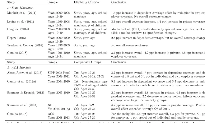
Unfortunately, there has not yet been a consensus on this question. Panel A of Table 1 briefly summarizes other work on the impact of the state mandates on health insurance coverage. Levine et al. (2011) and Gamino (2018) argue that the state mandates increased overall coverage, but Monheit et al. (2011) suggests they did not. Meanwhile, Depew (2015) and Trudeau and Conway (2018) found it depended on the model they implemented. This ambiguity regarding the impact of the state laws also flows into studies of the federal de-pendent coverage mandate. Cantor et al. (2012a) found that the ACA mandate had a much larger effect on individuals who were already eligible for dependent coverage via a pre-existing state mandate than it did for those for whom the ACA was their first chance to access de-pendent coverage. In contrast, Akosa Antwi et al. (2013) found that the ACA’s effect on dependent coverage of young adults was no different between states with and without their own mandates. This inconsistent state mandate literature is surprising considering that, as panel B of Table 1 summarizes, the literature on the ACA mandate’s effects on health insur-ance coverage has been largely in agreement. Cantor et al. (2012a), Sommers and Kronick (2012), Akosa Antwi et al. (2013), Sommers et al. (2013), and Gamino (2018) all argued the ACA had substantial effects on overall rates of coverage for young adults. One is left to wonder: why has the literature been unable to show consistently that the state mandates achieved their goal?
A few possible answers for this question have been offered by the literature. First, it has been noted by most authors that states have more limited authority to regulate health insurance plans than the federal government, which would explain tepid effectiveness found
1
by some authors. The states’ limited authority is due to the federal Employee Retirement Income Security Act of 1974 (ERISA), which exempts self-insured group plans from state regulation (Pierron and Fronstin, 2008). This explanation, however, fails to account for the popularity of the mandates among state governments, as more than half have adopted them over the last forty years. Why would they be so eager to adopt policies with limited effectiveness? Moreover, states have been shown able to affect other types of health plan benefits despite ERISA limitations (Gruber, 1994; Schmidt, 2007; Bitler and Schmidt, 2012; Bitler and Carpenter, 2016, 2017). A second possible explanation is information, as Cantor et al. (2012a) speculated that the state mandates made people more aware of the ACA, while Akosa Antwi et al. (2013) suggested they may not have understood the state mandates well. These arguments both seem difficult to justify. The ACA was well publicized following a societal and political debate on the topic leading up to its passage, so state policies seem unlikely to have been a major determinant to people’s awareness of it. Furthermore, the state mandates did not really require covered individuals to have much since information would naturally flow to members of affected health plans as their dependents did not automatically age out of coverage at 19. A third suggested explanation is difficulty in measurement, as the literature has noted that the results of Levine et al. (2011) and Monheit et al. (2011) are sensitive to data and specification choices, raising doubts about their validity (Burgdorf, 2014, 2015; Monheit et al., 2015; Gamino, 2018). Moreover, Depew (2015) and Trudeau and Conway (2018) found estimates were sensitive to the method used to classify who was eligible for state mandates.
In this study, we revisit the question of the effectiveness of the dependent coverage man-dates, and take steps towards resolving the ambiguity in the literature regarding their effects. We show that the state mandates did, in fact, achieve success at increasing overall health insurance coverage among those most likely to meet eligibility requirements and take up cov-erage. Moreover, the impact of the state mandates is also manifest in the effects of the federal mandate, which had less influence among those for whom the state mandates had already increased coverage. Among those not previously affected by the state mandates, though, we find large effects of the ACA mandate, and these are notably similar in magnitude to the effects found for the state laws.
past 40 years. This new dataset contains detailed information on the eligibility criteria and implementation dates for the complete history of the state mandates. Other authors have used data for the state mandates that contained numerous omissions and errors regarding when, where, and how the laws were adopted. The legal research our analysis relies on, however, substantially corrects these issues, allowing for improved measurement of mandate effects.2
Second, we analyze the effects of the mandates for separate age groups based on the insight that as young adults age, they quickly gain independence from their parents across numerous aspects of their lives. The more independent young adults are, the less likely they are to take up coverage through their parents’ health plans. Moreover, the state mandates often had eligibility criteria that were harder for individuals to satisfy as they gained independence. For example, most state laws required dependents to be unmarried. Consequently, we study these mandates across different age groups with the expectation that the youngest of the eligible individuals are most likely to be eligible and take up coverage. Our results show that (part of) the reason previous authors struggled to find effects of the state mandates was because they estimated combined effects between groups with strong im-pacts and others with small effects. The result was diluted estimates for the state mandates. Third, we depart from the bulk of the literature by avoiding reliance on endogenous per-sonal characteristics when identifying individuals who were eligible for coverage under state mandates. As noted by Depew (2015), relying on these characteristics reduces measurement error, but potentially introduces bias of an unknown character.
In sum, using our new data and analytical approach, we are able to provide a more com-prehensive understanding of the dependent coverage mandates, the extent of their efficacy, and the degree to which state and federal efforts interacted. The state mandates were effec-tive, but limited in their reach not because of limits to state regulatory power, but due to their greater dependency requirements. The ACA filled in to spaces the state mandates had not reached, affecting individuals who had not taken up previously available coverage due to eligibility restrictions, as well as those not previously covered by state mandates.
2
State and Federal Dependent Coverage Mandates
The federal government’s effort to address the high uninsurance rate of young adults began in March 2010 with the passage of the ACA. The ACA dependent coverage mandate allows young adults to remain eligible for coverage on their parents’ health insurance until they
2
reach age 26, without any restriction on marital, educational, residency, or dependency status. Though this was the first experience of many in the country with a dependent coverage mandate, the ACA was not entirely revolutionary. Instead, it was based on a blueprint set out by state efforts that had begun decades prior. Since the first such law, passed by Louisiana in 1974, the number of state-level expansions of dependent coverage has risen with increasing intensity, reaching 33 at the time of the ACA’s implementation (see Table 2).
Although the main motivation and the overall structure of the mandates are similar be-tween the federal and state mandates, they nonetheless have some important eligibility and implementation differences. For the case of the federal government’s mandate, eligibility applied to all young adults younger than 26 years old effective September, 2010. In contrast, the state mandates often have additional eligibility criteria, such as dependents having to be unmarried, students, living with their parents, or financially dependent on them. Addi-tionally, limiting ages – the ages under which young adults could be considered dependents on their parents’ health plans – have varied across states and time. In total, through the effective date of the federal mandate, there were 50 distinct enactments or material changes in state mandates. The history of these changes in limiting ages are summarized (through 2010) in Table 2. Two examples that illustrate the variety in eligibility criteria are Texas and South Dakota. Texas’ mandate first went operational in January 2002 with a limiting age of 25 and a requirement that dependents be unmarried. It has not changed since.3
South Dakota’s law, in contrast, has not remained static. Originally effective in July 2004, it had a limiting age of 24 and a requirement that dependents be full-time students. In 2007, the effective limiting age was further raised to 30 for students without another source for health insurance – except for those individuals born before July 1st
, 1983, for whom the increase did not apply.
The state mandate data we rely on from Barkowski and McLaughlin (2018) reflect state statutes that targeted the large group health insurance market, which is the dominant source of health insurance in the country, and has the most cost and tax advantages.4
To consider
3
Though the mandate has not been changed, the codification of Texas law underwent reorganization in 2005. This reorganization resulted from passage of a new bill in 2003, though its changes were not effective until 2005. This change probably explains why other authors incorrectly specified Texas’ mandate as going into effect on dates from 2003 through 2005.
4
a state to have a mandate, Barkowski and McLaughlin require it to have a statute setting a mandatory limiting age above 19 (as they take every state’s default limiting age as 19).5 They did not, however, include mandates allowing adult children with work-limiting dis-abilities to stay on their parents’ plans, since the vast majority of states had such laws and they applied to very small portions of the population. Their data were culled primarily from LexisNexis, HeinOnline, state government websites, and direct communication with state insurance departments or legislative analysts. Complete details on the laws and their interpretation can be found in the appendix to Barkowski and McLaughlin (2018).
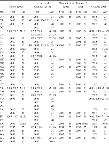
Table 2 presents a comparison of the maximum ages of eligibility (which is one year less than the limiting age) and years of expansion for state mandates according to the data we use, and those used by other authors investigating the effects of the state mandates on health insurance coverage (Levine et al., 2011; Monheit et al., 2011; Depew, 2015; Trudeau and Conway, 2018; Gamino, 2018). We find that there are significant differences between our legal data and those of these other studies.6
Louisiana and Connecticut provide two cases which illustrate some of the differences between our data and those of previous authors, and also serve as helpful examples of the language of state mandates. In the case of Louisiana, Levine et al. (2011) and Monheit et al. (2011) code the state as having no mandate, while Depew (2015) and Trudeau and Conway (2018) code it as having one starting in 2009, and Gamino (2018) has it beginning in 1997. We find, however, that it had one dating back to 1974 with a limiting age of 24, requiring a dependent be unmarried, a student, and financially dependent on his or her parents. Louisiana Revised Statutes§22:215.4, as effective July 12, 1974, provides the following:
[S]tudents who are unmarried children who have not yet attained the age of twenty-four and who are enrolled as full-time students at an accredited college or university, or at a vocational, technical, vocational-technical or trade school or institute, or secondary school, and who are dependent upon the primary insured under any group health and accident or franchise health and accident insurance policy issued in this state for their support, shall be considered as dependents under the provisions of said policy.
The law remained the same for the general population until 2010, when it was amended to mimic the ACA’s mandate. The fact that the mandate dated back so far may explain
5
There are at least a few cases where state statutes were passed that explicitly allowed extension of coverage to those above 19, but did not require it. One example is Virginia, which allowed expanded coverage starting in 1986, but did notrequire such coverage until 2011.
6
why Levine et al. (2011) and Monheit et al. (2011) were not aware of it. In 1997, the text of the statute was amended to ease eligibility for only those with mental health disabilities (and was not targeted at the general population), which probably explains the date given by Gamino (2018), while a reorganization of the state’s codification of laws in 2009 (which did not change the content of the statute) might be the reason for the date given by Depew (2015) and Trudeau and Conway (2018).
The mandate for Connecticut was enacted in 1976. Like Louisiana, this mandate was extended only to unmarried students who were still financially dependent on their parents, but had a lower limiting age of 23. From the General Statutes of Connecticut, Sec. 38a-554. (Formerly Sec. 38-374), as effective April 1, 1976:
A group comprehensive health care plan shall contain the minimum standard benefits prescribed in section 3 of this act, including the choice of the low option, middle option or high option deductible, and shall also conform in substance to the requirements of this section. (a) The plan shall be one under which the individuals eligible to be covered include: (1) Each eligible employee; (2) the spouse of each eligible employee; and (3) dependent unmarried children, who are under the age of nineteen or are full-time students under the age of twenty-three at an accredited institution of higher learning.
The statute remained the same until the limiting age was raised to 26 in 2007 when the student requirement was dropped and a state residency requisite was added. In 2009, the residency requirement was dropped, with no other changes, and in 2011 the limiting age was raised to 26 for children without their own employer provided insurance. As in the case of Louisiana, both Levine et al. (2011) and Monheit et al. (2011) code Connecticut as having no mandate and Depew (2015) and Trudeau and Conway (2018) code it with one since 2009. Gamino (2018) comes much closer, coding its beginning as 1982. The age of the statute was, once again, likely an influence in these mis-codings. Also similar to Louisiana, the relatively minor change to the law in 2009 is probably the cause of the 2009 record for the law held by Depew (2015) and Trudeau and Conway (2018).7
Beyond eligibility requirements and timing, another important difference between the federal and state mandates is that states’ abilities to regulate health plans are more limited than those of the federal government due to ERISA. According to statistics produced by the Agency for Healthcare Research and Quality using Medical Expenditure Panel Survey
7
data,8
as of 2010 in the USA, 35.8 percent of private-sector establishments offering health insurance self-insured at least one plan. For those with 50 or more employees, that figure is 63.3 percent. This suggests that a significant portion of the population may not have seen access expand due to state mandates. Despite this limitation on states’ authority, previous authors have shown that states have been able to influence health insurance benefits through mandates. These include maternity benefits (Gruber, 1994), infertility treatments (Schmidt, 2007; Bitler and Schmidt, 2012), and cancer screening (Bitler and Carpenter, 2016, 2017). Additionally, there is some reason to think that state mandates may influence health plans that are not explicitly subject to state authority. In particular, competition may induce firms to offer similar benefits in their health plans in order to attract quality employees. This theory is consistent with past research showing self-insured firm plans having similar benefits and costs as those that were not self-insured (Acs et al., 1996; Jensen et al., 1998; Gabel et al., 2003). Nevertheless, in the context of our study, the limitation to the states’ authority has an important implication: it leaves scope for the federal government’s ACA mandate to increase health insurance access to young adults, even in states with pre-existing mandates.
3
Empirical Strategy
3.1
Effects of State Mandates
The outcomes of interest in this study, indicated byH, are indicator variables for individual health insurance coverage via one of several different sources (such as public, private, or any). For our analysis of state mandates, our independent variable of interest isELIG, also an indicator, representing young adults’ imputed eligibility for health insurance coverage as dependents on their parents’ plans.9
We impute eligibility on the basis of survey respondents’ states of residence, ages, and interview years, assigning ELIG a value of one when all of those factors agree with our coding of a state mandate, and zero if not.
Since this coding scheme implies that ELIG varies across three dimensions, we estimate the impact of eligibility by implementing a triple differences (DDD) model. This approach allows us to identify the effect using within-state variation (across ages and time), while controlling for observable differences across those dimensions, measured using non-mandate states. In practice, this means our econometric models include a full set of two-way
fixed-8
See https://meps.ahrq.gov/data stats/summ tables/insr/state/series 2/2010/tiia2a.htm, viewed April 5, 2018
9
effects – age-by-state, age-by-year, and state-by-year – that control for trends across those dimensions in an unrestricted way. Thus, the identification assumption of our DDD model is that there were no other age-by-state-by-year variables that are correlated with imputed eligibility (that is, the state mandates) that also affect health insurance coverage.
Our model takes the following functional form:
Hiast=α+ρELIGast+γas+δat+µst+Xiast′ Θ +uiast, (1)
wherei,s,t, andaindex individuals, states, years, and ages, respectively. Xis a column vec-tor of individual and macroeconomic control variables, including dummies for gender, race, ethnicity, and metropolitan area classifications, plus age-year-state specific employment-to-population and poverty ratios. Race controls include white, black, Native American, Asian, Pacific Islander, other single race, and numerous additional multi-race indicators. Ethnicity controls include dummies for not Hispanic and several categories of Hispanic/Latino ori-gins. Metropolitan area classifications include central city, outside central city, unknown central city status, not in metro area, and not identifiable. We calculated our employment-to-population and poverty ratios using data from the American Community Survey and the 2000 Census 5% sample (ACS) (Ruggles et al., 2017), defining poverty as having family income below 150 percent of the federal poverty threshold. We estimated equation (1) via weighted least squares and clustered all standard errors at the state level.10
This model has the same primary features as ones implemented by Depew (2015) and Trudeau and Conway (2018).
Our imputation of eligibility for this model on the basis of only age, state, and year means that we are leaving aside the additional eligibility requirements of some state mandates, the most notable being marital and school enrollment requirements. This a key difference between our analysis and that of other authors (aside from Depew 2015 and Trudeau and Conway 201811
) who all use student or marital statuses (or both) as part of their imputation methods. We avoid using these since Depew (2015) argued they are potentially endogenous, an argument that was given empirical credence by previous work on marriage by Abramowitz (2016) and Barkowski and McLaughlin (2018). The disadvantage of this approach is that some individuals will be misclassified in our analysis, implying some attenuation in our estimates. We view this conservative approach as preferable to using the additional eligibility requirements, which would potentially introduce upward bias. This concern is also the
10
All regression parameter estimates and standard error are calculated using the “areg” and “cluster” option commands in Stata/MP 13.1 for Windows (StataCorp, 2013).
11
reason behind our choice to not include the other eligibility criteria as controls in our model. Moreover, we also do not include individual-level employment or income as controls, either, as Dillender (2014) suggests these also may be influenced by the state mandates.
We apply our econometric model to a sample of young adults who were the primary targets of the state expansions: those aged 19 to 29 years. As we noted above, though, these years in young adults’ lives are ones of significant transition where individuals rapidly become independent of their parents. Remaining part of parental health insurance plans is one form of parental dependence, particularly since many state mandates explicitly required residential or financial parental dependency. Other eligibility requirements, like being a student or unmarried, also imply less independence for young adults. Hence, we expect that the effects of the state mandates to be stronger among the younger individuals we study, since they are more likely to satisfy the dependency requirements of the laws and take up coverage through their parents. So, in addition to the 19 to 29 age group, we also apply our model to several subsamples of ages: 19 to 25, the age group targeted by the ACA mandate; 19 to 22; 23 to 25; and 26 to 29. This approach is another important difference between our study and that of the bulk other authors, and allows us to uncover a key factor in understanding the role of the state mandates played in the lives of young adults.
While the goal of the state mandates was clearly to increase health insurance cover-age, the manner in which they attempt to do this has implications for the sources by which young adults obtain their coverage. Since most parents obtain their health insurance through an employer, we expect that the mandates should increase coverage primarily through ex-panded employer provided dependent coverage.12
This may also have implications for other insurance sources, since dependent coverage may increase by crowding out other sources, as both Levine et al. (2011) and Monheit et al. (2011) previously argued. We, therefore, apply our model to several different insurance coverage sources, expecting the policies to directly increase dependent coverage types, but potentially decrease those available through independent sources, such as via young adults’ own jobs or public sources. For outcomes that aggregate coverage types, like private or coverage from any source, the expected effects are ambiguous, as they depend on the extent of crowd out.
A final aspect of our empirical strategy to identify the state mandate effects that needs to be discussed is the coding ofELIG. First, we note that enactment and effective dates of laws are often not the same date, so we are careful to consider effective dates when imputing
12
values for ELIG. Second, since the level of observation in this study is person-year, we need to assign all effective dates for mandates to the beginning of a year, even though the laws actually had various effective dates throughout the calendar year. Our approach is to assign all mandates with effective dates before July 1st as being effective for the whole year in which the mandate actually became effective. For mandates with effective dates July 1st or later, we assign the mandate as effective starting the beginning of the following year. This approach is intended to minimize the amount of misclassification taking place at the implementation of states’ policies.
3.2
Interaction of State and ACA mandates
The second focus of our study is the federal dependent coverage mandate, with particular at-tention on how pre-existing state mandates influenced its impact. Since the ACA’s mandate was implemented across all 19 to 25 year olds in the country at the same time, we cannot use our DDD strategy above to identify its effects, as the age-by-year fixed effects would absorb the ACA effects. We therefore use the difference-in-differences (DD) approach that has become standard in the ACA mandate literature (Cantor et al., 2012a; Akosa Antwi et al., 2013; Sommers et al., 2013). This strategy compares those targeted by the ACA mandate to a control group of older individuals who were not targeted by the ACA.13
We adapt this strategy to our context, using a model that allows us to estimate the effect of the federal dependent coverage mandate on those eligible for state mandates separately from those who are not. This model takes the form:
Hiast =α+β1ACAat ·P OSTt·ELIGast+β2ACAat·P OSTt+β3ACAat·ELIGast
+β4P OSTt·ELIGast+β5ELIGast+γas+µst +Xiast′ Θ +uiast, (2)
where the dummyACA identifies the young adults targeted by the federal mandate (the 19 to 25 year olds, inclusive) and P OST indicates years after 2010 – the effective years of the federal mandate. The definitions of other variables are the same as in equation (1), with X
containing the same set of control variables. This model has the same basic form as that of Cantor et al. (2012a), with our stronger controls for trends (state-by-year and state-by-age) and method of coding ELIG being the key differences.
Equation (2) has two primary parameters of interest,β1andβ2, which allow us to measure
13
three relevant quantities. The first of these, represented by β2, is the DD effect of the ACA on young adults not eligible for coverage via state mandates. This reflects the comparison of individuals aged 19 to 25 to those above 25, among those not eligible for any state mandate. The second quantity, represented by β1 +β2, is the effect of the ACA on state mandate eligible young adults, and also reflects a DD comparing the older and younger individuals, though this time only among those eligible for state mandates. The final object of interest is β1, the difference between the first two quantities. We report estimates for each of these quantities in our discussion of our results, below.
We apply equation (2) to three different age groups. The first is those aged 19 to 28, inclusive. Our exclusion of age 29 individuals is a departure from our state mandate analysis; we make this change to increase the similarity of the control group of individuals above 25 to the younger treatment group. The second group is comprised of ages 19 to 22 and 26 to 28, and excludes 23 to 25 year olds to isolate the effect on the younger individuals targeted by the federal mandate. Finally, the third group is those aged 23 to 28, which enables us to estimate the effect solely on the 23 to 25 year olds.14
Splitting our analysis across these age groups allows us to complement our state inquiry and see whether ACA effects were heterogeneous across ages, and how state effects on age subgroups interacted with the ACA. We expect that if the state mandates were successful in increasing insurance coverage for a subgroup, then the impact of the ACA would be attenuated for that group, since it would not be introducing any actual treatment.15
Finally, before moving to a discussion of our data, we note that our coding of the P OST
variable implies an effective date of the ACA as the start of 2011, despite its true effective date being in 2010. Since our data is annual, we could only chose the beginning of 2010 or 2011 to model the law’s implementation, and the choice of 2011 is consistent with how we coded state mandate effective dates, since the ACA officially became effective after July 1st, 2010.
14
We also analyzed a sample of 19 to 28 year olds that excludes 26 year olds, as 26 is the transition age between eligibility for the ACA mandate or not, as a robustness check. The results were quantitatively and qualitatively similar, if not slightly stronger, than the base case we report.
15
4
Data
We apply our empirical strategies laid out above to a sample of data on health insurance coverage from the Annual Social and Economic Supplement (ASEC) of the Current Popu-lation Survey (CPS) for the survey years 2001 through 2013 (Flood et al., 2017). Coverage questions in this survey are retrospective, so refer to years 2000 through 2012. In robustness checks, we extend our sample back to reference year 1990 (survey year 1991) for outcomes where data availability allows, and for the rest back to reference year 1996 (sample year 1997). For our study of the state mandates before the implementation of the ACA, we end our sample in reference year 2010 so as to exclude the federal mandate’s influence. For our analysis of the interaction of both state and federal mandates, however, we do not end our sample until reference year 2012 (survey year 2013), after which the health insurance questions in the CPS underwent significant redesign. We start our primary sample for both analyses in reference year 2000 to coincide with the availability of annual data from the ACS and the 2000 census, which we use for measures of employment and poverty (Ruggles et al., 2017). In our extended sample, reference year 1990 was chosen as start date to corre-spond with the period in which we had coded our state mandate data into database format. Hereafter, when we refer to a year of our data, we mean the reference year unless otherwise stated.
We chose the CPS for our analysis because of its long and (relatively) consistent history as a survey of health insurance coverage, and because it offers significant detail regarding coverage source. These characteristics have made it popular among researchers, as it is widely used for estimates of insurance coverage. Nevertheless, there are some difficulties related to using this survey for our analysis. One of these is survey non-response, which was typically above 15 percent during the period covered by our sample (for example, see the Source and Accuracy Statement for U.S. Bureau of the Census, 2005). While the Census Bureau imputes data for these observations, we exclude them from our analysis and use the weight variable developed by the State Health Access Data Assistance Center (SHADAC) for use with their summary CPS health insurance variables, which adjusts for the dropped non-response observations. We use the SHADAC summary health insurance variables in place of the original CPS variables when possible, but we use the same SHADAC weight in either case.16
Another potential concern with the CPS is measurement error. Many studies have shown that the uninsurance rate in the CPS is systematically higher than that measured by other
16
The SHADAC summary health insurance variables address other issues found in the original health insurance variables, as well. More information can be found in the documentation for these variables at
surveys (Swartz, 1986; Bennefield, 1996; Bhandari, 2004; Ham and Shore-Sheppard, 2005). One possible reason for this is the retrospective perspective of the survey, which asks re-spondents between February and April about coverage during the entire previous calendar year. This results in a long recall period for respondents, which may result in underre-porting of short coverage spells (Bhandari, 2004). In our view, though, this issue is more indicative of an interpretation problem than measurement error. We argue that, instead of measuring coverage at any point during the previous year, the CPS measures coverage at a point-in-time closer to the date of the interview, as has been previously suggested by Swartz (1986). This view is supported by research undertaken by the Census Bureau before implementation of the health insurance redesign. During the 2013 ASEC interview cycle, the Census Bureau implemented the original health insurance questions and the redesigned ones on parallel samples of individuals. This allowed them to estimate health insurance coverage using the traditional approach as well as a method representing a time-of-interview estimate and a method more clearly referencing coverage during the previous calendar year. The traditional method estimates resulting from this were much closer to the time-of-interview estimates than the new calendar year ones (Pascale et al., 2016). Nevertheless, we do not fully abandon the retrospective interpretation, since the survey does reference the previous year. Instead, we interpret the CPS as measuring coverage approximately at the end of the previous year. Given that health insurance is highly serially correlated within individuals, in our view this reconciles the results obtained by (Pascale et al., 2016) with the retrospective framing of the survey.
The interpretation of health insurance questions in the CPS is significant for this study because it informs our treatment of respondents’ ages, which influence the values taken by
5
Results
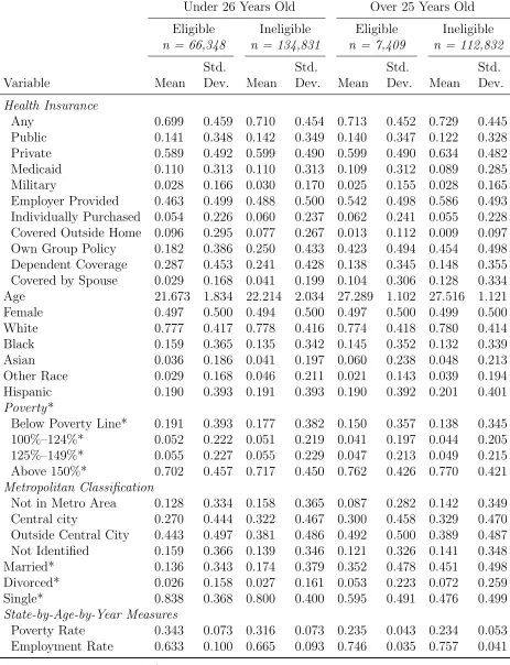
Before discussing our main results, we first report basic characteristics of our sample. Table 3 presents descriptive statistics of our data split into four sub-groups: under 26 years old and eligible or not for state mandates, and over 25 and eligible or not. The first two groups are used in our first, pre-ACA state mandate analysis, while all four are used in our state/federal interactions analysis. In general, we observe similarities across the four groups for any health insurance, public, private, Medicaid, Military, Medicare, and individually purchased health insurance. Having any health insurance is slightly more likely for those who are ineligible and 26 years or older. We observe large differences across four groups for employer provided coverage, own group policy, and covered as a dependent. Having coverage as a dependent is more likely for the younger age group, particularly for those eligible under state laws. Complementing this, we note that the older individuals are more likely to have their own policies, as do younger ones ineligible under state laws. Gender, race, and ethnicity are similar across groups, while the older groups have higher incomes on average, as would be expected. Metropolitan classification shows some differences across groups, with eligible individuals being more likely to be located outside of a central city area, and ineligible individuals being more likely to not be in a metropolitan area at all. Marital status also reflects expected differences across age, with older individuals being much more likely to be married or divorced.
5.1
Effects of State Mandates
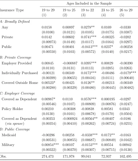
Estimates of equation (1) based on our sample for the years 2000 through 2010 are reported in Table 4. We also present a set of estimates based on our extended sample for the years 1990 or 1996 through 2010, reported as a robustness check, in Appendix Table 1.17
As we discuss below, our estimates are similar in both sample periods. All cells in the tables report estimates for ρproduced by separate regressions which differ on the basis of the outcomes or samples used, as indicated by the row and column headers. All estimates reported in these tables should be interpreted as percentage point changes (for example, 0.01 represents a one percentage point increase) in health insurance coverage attributable to eligibility for a state mandate.
17
We begin with column (1) of Table 4, where we report results for the full range of ages in our sample, 19 through 29. Effects on this age range overall are weak, though we note that we estimate dependent coverage to increase by almost a percentage point, and coverage outside the home to increase by half a percentage point, both of which are significant (p <0.1). The CPS does not specifically identify the source of health insurance outside the home, but the nature of coverage outside the home implies it would be some sort of dependent coverage – likely parental since spouses usually live together. Thus, both of these results are consistent with the expected effects of the mandates. Most of the other estimates are not statistically significant at conventional levels of significance, but our point estimates for private coverage and coverage from any source both are about one-and-a-half percentage points, results that are consistent with the dependent coverage estimates. For an unclear reason, we also obtain a statistically significant increase in military insurance coverage of about 0.9 percentage points, though this result is much smaller and insignificant in our extended sample (Appendix Table 1). Other estimates in our extended sample are similar in most cases.
Among the other work in the literature, the figures reported in column (1) are most comparable to estimates produced by Depew (2015) and Trudeau and Conway (2018), since both authors used CPS samples of 19 through 29 year olds, used similar DDD models, and imputed eligibility via age, state, and year. Depew reports a 2.3 percentage point increase in parental dependent coverage, and a one percentage point increase in any insurance, the latter of which is not statistically significant. Since Depew’s measure of dependent coverage specifically identifies coverage through a parent and includes coverage outside the home in this measure (which we separate out), his results are fairly consistent with ours. Trudeau and Conway (2018) report only an estimate for any insurance, finding an insignificant increase of 0.4 percentage points. Both our main and extended sample estimates are bigger than this, but neither is significant. Our results for any coverage, therefore, generally agree with estimates from both previous studies.18
Column (2) reports results for the age range 19 to 25, the target ages of the federal man-date. Here we find a set of estimates that is often similar to the ones in column (1), though none of these results are statistically significant, and some figures suggest weaker effects. In particular, estimates for private or any coverage are both about half the size as in column (1). On the other hand, the strongest estimates from column (1), dependent and coverage outside the home, are notably similar in magnitude in column (2). Several other authors (Levine et al., 2011; Monheit et al., 2011; Trudeau and Conway, 2018; Gamino, 2018) have
18
reported estimates for a similar age range (19 to either 24 or 25), though the appropriateness of comparison is unclear because, in addition to different sample year ranges and different mandate codings, each of these has included student or marital status requirements, or both, as part of their eligibility imputations. Generally, these analyses return stronger estimates than ours, with Levine et al. (2011), Trudeau and Conway (2018), and Gamino (2018) each finding effects on any coverage of around three percentage points. Monheit et al. (2011) found increased dependent coverage crowded out coverage through own employers, resulting in no significant effects on overall coverage. Thus, for this type of sample our results are quite different from other studies, but this is unsurprising given the data and methodological discrepancies between the studies.
To this point, our estimates obtained using corrected legal data show weak evidence of effects for the state mandates. However, when we restrict our sample to ages 19 through 22, as in column (3), the results are drastically different. For this subsample, we estimate a statistically significant (p < 0.01) increase of approximately 5.8 percentage points for dependent coverage. This represents a sizable effect of about 17 percent when compared to this subsample’s dependent coverage rate of 34 percent. Additionally, we find a significant increase in coverage outside the home of 1.3 percentage points (p < 0.05). Since our measure of dependent coverage includes both parental and spousal coverage, we note that we also estimate a small, but statistically significant, reduction in spousal dependent coverage (p <
0.05), which is consistent with some individuals trading off spousal for parental coverage (Abramowitz, 2016; Barkowski and McLaughlin, 2018). This spousal coverage estimate also suggests our results are not subject to the critique levied by Burgdorf (2014, 2015) against Monheit et al. (2011), that their model found effects through spousal coverage, not parental, a result inconsistent with the policy’s legal mechanism. Combined, dependent coverage and coverage outside the home account for the substantial portion of the significant 7.4 percentage point increase (p < 0.01) in private coverage we estimate.
percentage points (p < 0.01).19
While at first glance one might be surprised to see an effect on military coverage, such a result is consistent with young adults substituting parental for employment coverage, something other authors have suggested was plausible (Monheit et al., 2011). Additionally, our significant 1.7 percentage point estimate (p < 0.01) for individual coverage might be unexpected, but we argue this result is not implausible. While our research on the state laws focused on group dependent coverage mandates, many states’ mandates had scopes that were broader than just group coverage. Our interpretation of this estimate is, therefore, that young adults were added to their parents’ individually purchased plans as dependents. With regard to the estimates from our extended sample in Appendix Table 1, we find that most are similar to our main results. Two notable differences are those for individual and outside home coverage. The first of these does not have a significant effect in the extended sample, while the second estimate is a significant decrease of 1.5 percentage points. While we do not have any insight as to why we observe these changes, we note that private and overall coverage estimates do not reflect the full differences observed in these outcomes.
With one exception, other authors in this literature have not studied any sub-groups younger than the 19 to 24 year old groups, so comparison with other authors’ work is difficult for this sample. The only exception, Burgdorf (2014), replicated the model used by Levine et al. (2011) and then used it to produce separate estimates for each age within the 19 to 24 group. These estimates were sensitive to model and sample specifications and not uniformly statistically significant, but the point estimates were generally larger for the younger ages. This is roughly consistent with our findings, even if the differences in data and analytic approaches make comparison tenuous.
We move next to estimates where the sample is restricted to ages 23 through 25, presented in column (4). For this range of ages, we find little evidence of mandate effects. Only two of our outcomes show estimates that are significant at conventional levels, and these are directly related to each other. In particular, the estimate for Medicaid is a positive 1.7 percentage points (p <0.05), and this is reflected in the significant 2.4 percentage point result for public coverage (p <0.1). One possible explanation for this surprising result is that the adoption of some state mandates took place simultaneously with expansions to state Medicaid programs. These Medicaid changes took place from the late 1990s through the mid-2000s and increased Medicaid coverage for individuals over age 20 (Hamersma and Kim, 2013). On the other hand, the Medicaid estimate on our extended sample (Appendix Table 1) is essentially zero. Instead, military coverage is significant along with public coverage overall (though
19
public is smaller than in the main sample). Hence, these results may be originating from measurement variability or other issues. Among the various forms of private coverage where we would most expect to observe effects, we generally obtain estimates that are quite small, with only employer provided and any coverage having even moderate magnitudes (and the result for any coverage likely reflects the estimated increase in public). Nevertheless, we note that while our results rule out strong effects, it is possible that the mandates could have had small to moderate effects that our study does not have the precision to identify. For example, on dependent coverage, the 95% confidence interval includes effects above 1.7 percentage points. Nevertheless, even if some effects are being overlooked here, it is clear that the 23 to 25 year olds were less affected by the state mandates than the 19 to 22 year olds.
Column (5) contains estimates for our subsample of 26 to 29 year olds. Generally, our results for this group are very noisy, resulting in only one statistically significant estimate, individually purchased insurance. Here we find it fell by 1.8 percentage points (p < 0.01). One possible reason for such a result would be crowd out from another source. While we have no other significant results, we note that our estimate for employer coverage as the policy holder is positive in this sample. These two estimates would be consistent with eligible individuals transitioning from coverage on individual plans to those through their own jobs, though why such a result would be induced by mandates is unclear. Thus, the overall pattern of estimates for this subsample is not consistent with a state mandate influence, though their imprecision means that we cannot rule out a moderate-sized impact. This is also true for our extended sample, where our results share most of the same characteristics of our main sample – the point estimates are similar and are also generally imprecise. Unfortunately, we do not have any other estimates from other papers in the literature to compare these results to, since as far as we know, ours are the first estimates in the literature based on the 26 to 29 age group.
mandates’ split effectiveness. The second goal is to see whether the effects of the state mandates directly interacted with those of the ACA. To do so, we design our analysis to tell us whether the groups most strongly affected by the state mandates were influenced differently by the ACA than other groups. This will provide more context into how state and federal mandates work when they simultaneously target similar populations and have similar policy goals. Given our results above, our hypothesis is that the effect of the ACA should be attenuated among the 19 to 22 year olds since that group already had health insurance due to the state mandates.
5.2
Interaction Effects
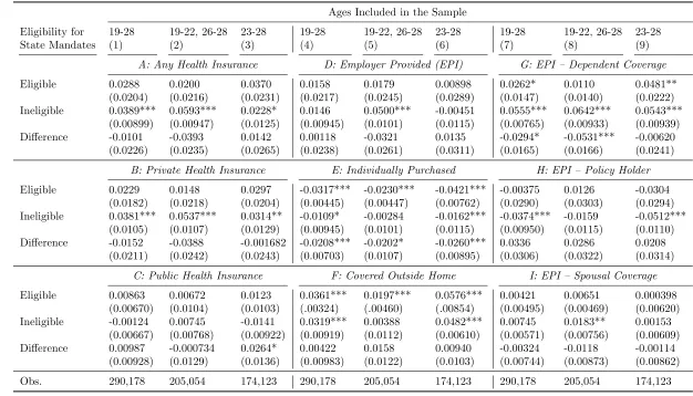
Table 5 reports estimates of employer provided health insurance coverage effects based on equation (2). In contrast to our pre-ACA, state-mandate analysis, which reports results for eleven outcomes, for space reasons we present for only nine here. The omitted outcomes are Medicaid and military coverage, which we chose to exclude since they are measured closely by the public category. Also differing from our state analysis is the time period of our sample, which consists of years 2000 through 2012, allowing us to observe two full years after the implementation of the ACA’s federal mandate. Our sample is, therefore, much longer than those of the other authors in this literature. Additionally, we again present a robustness check based on our extended sample that covers the years 1990 or 1996 through 2012 in Appendix Table 2.20
Our estimates from this extended sample substantially mimic our main results. Both tables contain separate panels for each of the nine outcomes, and within each panel are results from three independent regressions – one for each age subsample. We present estimated effects for both the eligible and ineligible, as well as the difference between the two. These represent estimates of β1 +β2, β2, and β1 from equation (2), respectively. As before, all estimates reported in these tables should be interpreted as percentage point changes in health insurance coverage – in this case attributable to eligibility for the federal mandate.
We begin by comparing our estimates for overall coverage for our broadest sample to those of other authors in the literature. Panel A, column (1) of Table 5 presents these results. We find the ACA increased coverage for the ineligible by 3.9 percentage points, a statistically
20
significant result (p < 0.01), while our 2.9 percentage point estimate for the eligible is not significant at conventional levels. The difference between these estimates is also not significant. Of the other studies on the ACA mandate, only Cantor et al. (2012a) produced estimates by eligibility status, finding a 3.8 percentage point increase in any coverage for the ineligible, and (a surprising) 8.3 for the eligible. Gamino (2018) produced estimates for the ACA effect on the ineligible only, finding a 5.5 percentage point increase. Other authors produced estimates only for pooled statuses, with their results ranging from 2.9 to 4.7 percentage points (see panel B of Table 1 for a summary). Thus, our estimates are consistent with the rest of the literature in noting that the ACA was effective in raising overall coverage for young adults. Our overall estimates are distinct, however, in obtaining a larger estimate for those who were ineligible for state mandates.
The rest of the estimates presented in Table 5 provide significant insight into how the ACA effected the increase we find overall. Looking first at panel G, we find it induced an interesting pattern of change in dependent coverage. For the 19 to 28 age group in column (7), we estimate a much larger increase in dependent coverage for those who were ineligible than for the eligible. Both groups saw statistically significant increases, but the effect for the ineligible at 5.6 percentage points (p < 0.01) was more than double that of the eligible at 2.6
(p <0.1). The 2.9 percentage point difference between the two is also significant (p <0.1).
The estimates in the next two columns, however, show that the single estimate across ages hides important heterogeneity. For 19 to 22 year olds, the ACA effect estimated in column (8) is large for the ineligible, but much smaller and insignificant for the eligible – precisely where the state mandates had been most impactful. On the other hand, among the 23 to 25 year olds in column (9), the ACA had similar sized effects for both the eligible and not. This supports the argument that restrictive eligibility requirements are the reason the state mandates did not have broader impact – not ERISA’s restrictions on state-level regulatory authority. It is also worth noting that our significant point estimates here are remarkably similar to those we obtained for the state mandate effect on 19 to 22 year olds. That is, for dependent coverage, whenever we find a significant effect, the estimate magnitude is consistent, regardless of whether the policy was state or federal in nature.
year olds, for whom our estimates are effectively zero. While this estimate represents only a small portion of the overall estimate for dependent coverage, we nevertheless took a closer look at this result by re-estimating equation (2) after dropping the 28 year olds from our sample. We take this step seeking to increase the similarity of the treatment and control groups. When doing so, the significant result decreases in magnitude to 1.3 and becomes insignificant. However, the estimate for 19 to 22 eligible young adults becomes significantly positive at 1.2 percentage points. In contrast, our estimates for dependent coverage and any health coverage are both similar whether we include the 28 year olds in the sample or not. Thus, we are inclined to view the spousal coverage result we report in panel I with skepticism given its comparative sensitivity to the sample. Whatever the case, though, given the magnitude of our dependent coverage results, it is clear they are not driven by spousal coverage.
Moving next to panel D, employer provided insurance, we see that the effect on dependent coverage for the ineligible 19 to 22 year olds is reflected here, though the effect seen for the 23 to 25 year olds is not. In the CPS, the employer provided coverage outcome aggregates the dependent (panel G) and policy holder (panel H) measures, so the reason we do not see effects for the older group in employer coverage overall is because the increased dependent coverage for this group crowded out coverage through the young adults’ own jobs. For ineligible 23 to 25 year olds, dependent coverage increased 5.4 percentage points while employer coverage as the policy holder decreased by 5.1 (both p < 0.01). Similarly, for the eligible, the 4.8 percentage point increase in dependent coverage was offset by a decrease of 3 percentage points in being the policy holder directly. Though this decrease was not significant, it still resulted in the net effect on employer coverage being small and insignificant, despite the large increase in dependent coverage. Among the 19 to 22 year olds, we find no evidence of the crowd out of own policy coverage, with the natural explanation being that these young adults are the least likely to have jobs that offer health insurance.
dependent coverage,21
so we are not surprised to find the larger increases are concentrated among the older group, since they are more likely to live outside their parents’ homes. We next note that for individually purchased plans (panel E) we find statistically significant coveragedecreases for each of the groups that saw increased outside home coverage, a result consistent with young adults trading off individual plans for coverage through their parents’ plans. Looking at the underlying components of private coverage as a whole, we note that the federal mandate induced substantial increases in coverage as a dependent (whether outside the home or not) for groups that did not see big increases under the state mandates. For the older individuals, however, this dependent coverage increase induced substantial crowd out of plans obtained through young adults’ own employers or individually. For the younger individuals, though, there was much less crowd out, primarily since those individuals did not have jobs through which to obtain insurance. On net, then, we see the largest increases in private coverage among the 19 to 22 year olds who were ineligible for state mandates.
Turning next to public health insurance in panel C, we present estimates that are gener-ally small, with none statisticgener-ally significant. We find this result somewhat surprising, given our results on the state mandates which showed significant crowd out of public plans among the 19 to 22 year old age group. For the older group of individuals, this finding can be largely attributed to the ACA’s dependent coverage effect crowding out other private sources, rather than public ones. But for the ineligible 19 to 22 year olds, the lack of crowd out of public sources means we essentially observe no crowd out at all among any alternative sources for this group. Overall, our lack of effects found for public coverage means that our results for any coverage in panel A essentially reflect net changes in private coverage only. Consistent with this, our estimates in panel A closely resemble those found for private coverage in panel B.
6
Conclusion
In this study, we performed a comprehensive analysis of the effects of both state and federal dependent coverage mandates on health insurance coverage of young adults. Our investiga-tion is unique in the literature in that we bring together three important analytical features: newly available, accurate data on the state mandates; a focus on heterogeneity across age groups likely to differ in their dependence on their parents; and avoidance of endogenous individual characteristics when imputing eligibility for state mandates. Our results provide
21
new insights on the effectiveness of the state mandates, how they interact with the ACA, and how differences in their designs might explain variation in their effectiveness. For the state mandates, we found they significantly increased dependent and overall coverage rates among young adults between ages 19 and 22. We also found evidence this new dependent coverage was partially offset due to crowd out of public health insurance. In contrast, we find little evidence of changes in coverage for 23 to 25 year olds. It is possible there was some effect of these mandates that we are simply unable to detect, but our results strongly point to larger effects for the younger individuals in our sample. We argue this dichotomy is consistent with young adults gaining independence as they age, making them less likely to take up coverage with eligibility requirements that limit this independence. With regard to the ACA, we present strong evidence that its effects were not uniform. We find it increased dependent coverage for all groups except those whom had been most strongly affected by the state mandates – eligible 19 to 22 year olds. This increase in coverage flows through to overall coverage, though less so for 23 to 25 year olds, as they also became less likely to hold their own, employer-provided policies or private coverage from the individual market. Since young adults ages 19 to 22 are less likely to hold jobs that offer health insurance, we find much less evidence among them for this type of coverage crowd out. In contrast to our results for the state mandates, we find no evidence that the ACA crowded out public coverage.
From these results, we draw three broad conclusions. First, our results provide strong evidence that the states were able to effect changes in health insurance coverage despite ERISA limits on its regulatory authority, a finding consistent with evidence found by authors studying other types of mandates (Gruber, 1994; Schmidt, 2007; Bitler and Schmidt, 2012; Bitler and Carpenter, 2016, 2017). To the extent that researchers have found effects of the state mandates difficult to pin down, this has more to do with having correct data on the mandates and identifying the population of people likely to take-up coverage than it does with ERISA. Second, we find that the ACA had a much smaller impact where the state mandates had the most influence. This is clear evidence of interactive effects in a case where state and federal mandates simultaneously target the same populations. This suggests that researchers studying overlapping policies – especially those on health insurance coverage – should be careful to account for state and federal policy interplay. Third, we found the state mandates were clearly effective for younger individuals, and less so for older ones, while the ACA did not seem to be limited in its scope by age. In our view, this suggests that the eligibility restrictions imposed by the states were the driving force behind their reduced impact among the older individuals they targeted.
References
Abramowitz, Joelle, “Saying, ”I Dont”: The Effect of the Affordable Care Act Young Adult Provision on Marriage,” Journal of Human Resources, October 2016, 51 (4), 933– 960. 10, 18
Acs, Gregory, Stephen H. Long, M. Susan Marquis, and Pamela Farley Short, “Self-Insured Employer Health Plans: Prevalence, Profile, Provisions, and Premiums,”
Health Affairs, January 1996, 15 (2), 266–277. 9
Antwi, Yaa Akosa, Asako S. Moriya, and Kosali Simon, “Effects of Federal Policy to Insure Young Adults: Evidence from the 2010 Affordable Care Act’s Dependent-Coverage Mandate,” American Economic Journal: Economic Policy, November 2013, 5 (4), 1–28. 3, 4, 12, 30
Barkowski, Scott and Joanne Song McLaughlin, “In Sickness and in Health: The Influence of State and Federal Health Insurance Coverage Mandates on Marriage of Young Adults in the USA,” Working Paper, Social Science Research Network January 2018. 4, 5, 6, 7, 8, 10, 18
Bennefield, Robert, “Comparative Analysis of Health Insurance Coverage Estimates: Data from CPS and SIPP,” Working Paper 9608, U.S. Census Bureau 1996. 15
Bhandari, Shailesh, “People with Health Insurance: A Comparison of Estimates from Two Surveys,” Working Paper 243, U.S. Census Bureau 2004. 15
Bitler, Marianne P. and Christopher S. Carpenter, “Health Insurance Mandates, Mammography, and Breast Cancer Diagnoses,” American Economic Journal: Economic Policy, August 2016, 8(3), 39–68. 4, 9, 25
and , “Effects of State Cervical Cancer Insurance Mandates on Pap Test Rates,” Health Services Research, February 2017,52 (1), 156–175. 4, 9, 25
and Lucie Schmidt, “Utilization of Infertility Treatments: The Effects of Insurance Mandates,” Demography, February 2012,49 (1), 125–149. 4, 9, 25
Burgdorf, James R., “Young Adult Dependent Coverage: Were the State Reforms Ef-fective?,” Health Services Research, December 2014, 49 (S2), 2104–2128. 4, 11, 18, 19, 30
, “Young Adult Dependent Coverage: Were the State Reforms Effective? A Critique and a Response,” Health Services Research, June 2015, 50(3), 637–641. 4, 18
Cantor, Joel C., Alan C. Monheit, Derek DeLia, and Kristen Lloyd, “Early Im-pact of the Affordable Care Act on Health Insurance Coverage of Young Adults,” Health Services Research, October 2012,47 (5), 1773–1790. 3, 4, 12, 13, 22, 30
Depew, Briggs, “The effect of state dependent mandate laws on the labor supply decisions of young adults,” Journal of Health Economics, January 2015, 39, 123–134. 3, 4, 5, 7, 8, 10, 17, 30, 31
Dillender, Marcus, “Do more health insurance options lead to higher wages? Evidence from states extending dependent coverage,” Journal of Health Economics, July 2014, 36, 84–97. 7, 11
Flood, Sarah, Miriam King, Steven Ruggles, and J. Robert Warren, “Integrated Public Use Microdata Series, Current Population Survey: Version 5.0.,” Technical Report, University of Minnesota, Minneapolis 2017. 14
Gabel, Jon R., Gail A. Jensen, and Samantha Hawkins, “Self-Insurance In Times Of Growing And Retreating Managed Care,” Health Affairs, March 2003, 22(2), 202–210. 9
Gamino, Aaron, “New Evidence on the Effects of Dependent Coverage Mandates,” Work-ing Paper, Social Sciences Research Network March 2018. 3, 4, 7, 8, 17, 18, 22, 30, 31
Gruber, Jonathan, “The Incidence of Mandated Maternity Benefits,”The American Eco-nomic Review, 1994,84 (3), 622–641. 4, 9, 25
Hahn, Youjin and Hee-Seung Yang, “Do Work Decisions among Young Adults Respond to Extended Dependent Coverage?,” ILR Review, May 2016, 69 (3), 737–771. 7
Ham, John C. and Lara Shore-Sheppard, “The effect of Medicaid expansions for low-income children on Medicaid participation and private insurance coverage: evidence from the SIPP,”Journal of Public Economics, January 2005, 89 (1), 57–83. 15
Hamersma, Sarah and Matthew Kim, “Participation and crowd out: Assessing the effects of parental Medicaid expansions,” Journal of Health Economics, January 2013, 32
(1), 160–171. 19
Jensen, Gail A., Kathryn Rost, Russell P.D. Burton, and Maria Bulycheva, “Mental health insurance in the 1990s: are employers offering less to more?,” Health Affairs, May 1998, 17 (3), 201–208. 9
Levine, Phillip B, Robin McKnight, and Samantha Heep, “How Effective are Public Policies to Increase Health Insurance Coverage Among Young Adults?,” American Eco-nomic Journal: EcoEco-nomic Policy, February 2011,3 (1), 129–156. 3, 4, 7, 8, 11, 15, 17, 18, 19, 30, 31
Monheit, Alan C., Joel C. Cantor, and Derek DeLia, “Drawing Plausible Inferences about the Impact of State Dependent Coverage Expansions,” Health Services Research, June 2015, 50(3), 631–636. 4
Pascale, Joanne, Michel Boudreaux, and Ryan King, “Understanding the New Cur-rent Population Survey Health Insurance Questions,”Health Services Research, February 2016,51 (1), 240–261. 15
Pierron, William L. and Paul Fronstin, “ERISA Pre-emption: Implications for Health Reform and Coverage,” Technical Report 314, Employee Benefit Research Institute Febru-ary 2008. 4
Ruggles, Steven, Katie Genadek, Ronald Goeken, Josiah Grover, and Matthew Sobek, “Integrated Public Use Microdata Series, American Community Survey: Version 5.0.,” Technical Report, University of Minnesota, Minneapolis 2017. 10, 14
Schmidt, Lucie, “Effects of infertility insurance mandates on fertility,” Journal of Health Economics, May 2007, 26 (3), 431–446. 4, 9, 25
Sommers, Benjamin D. and Richard Kronick, “The Affordable Care Act and Insurance Coverage for Young Adults,”JAMA, March 2012, 307(9). 3, 30
, Thomas Buchmueller, Sandra L. Decker, Colleen Carey, and Richard Kronick, “The Affordable Care Act Has Led To Significant Gains In Health Insurance And Access To Care For Young Adults,”Health Affairs, January 2013, 32 (1), 165–174. 3, 12, 30
StataCorp, “Stata Statistical Software: Release 13.1,” 2013. 10
Swartz, Katherine, “Interpreting the estimates from four national surveys of the number of people without health insurance,”Journal of Economic and Social Measurement, 1986,
14(3), 233–242. 15
Trudeau, Jennifer and Karen Smith Conway, “The Effects of Young Adult-Dependent Coverage and Contraception Mandates on Young Women,”Contemporary Economic Pol-icy, January 2018, 36(1), 73–92. 3, 4, 7, 8, 10, 17, 18, 30, 31
Table 1: A Brief Summary of Studies on Dependent Coverage Mandate Effects on Health Insurance Coverage
Study Sample Eligibility Criteria Conclusion
A: State Mandates
Monheit et al. (2011) Years 2000-2008 Ages 19-29
State, year, age, school, marriage
1.5 ppt increase in dependent coverage offset by reduction in own em-ployer coverage. No overall coverage change.
Levine et al. (2011) Years 1999-2008 Ages 19-24
State, year, age, school, marriage, # of children
3.3 ppt overall coverage increase, 4.4 ppt increase in private coverage.
Burgdorf (2014) Years 2000-2008 Ages 19-29
State, year, age, school, marriage, # of children
Monheit et al. (2011) results driven by spousal coverage. Levine et al. (2011) results sensitive to specification changes.
Depew (2015) Years 2000-2009 Ages 19-29
State, year, age 2.3 ppt increase in dependent coverage, but no overall coverage change.
Trudeau & Conway (2018) Years 1997-2009 Ages 19-29
State, year, age No overall coverage change.
Gamino (2018) Years 1996-2010 Ages 19-24
State, year, age, school, marriage
3.7 ppt increase overall, 4.2 ppt increase in private, 5.6 ppt increase in employer coverage.
Study Sample Comparison Groups Conclusion
B: ACA Mandate
Akosa Antwi et al. (2013) SIPP 2008 Panel Years 2008-2011
Trt: Ages 19-25 Ctl: Ages 16-18, 27-29
3.2 ppt increase overall, 7 ppt increase in dependent coverage, and de-creases of 0.8 ppt and 3.1 ppt in individual and own employer coverage. Cantor et al. (2012a) Years 2004-2010 Trt: Non-students ages
19-23 and all aged 24-25 Ctl: Ages 27-30
5.3 ppt increase in dependent coverage and 3.5 ppt decrease in unin-surance, with effects much larger in states with their own mandates.
Sommers & Kronick (2012) Years 2005-2010 Trt: Ages 19-25 Ctl: Ages 26-34
2.9 ppt increase overall, 2.8 increase in private, 4.3 ppt increase in de-pendent coverage, and 2.5 decrease as policy holder. Effects on overall coverage were larger for minority groups.
Sommers et al. (2013) NHIS
Yrs 2005-2011q3
Trt: Ages 19-25 Ctl: Ages 26-34
4.7 ppt increase overall, 5.1 ppt increase in private coverage. Positive overall effect extended through Q3 of 2011.
Gamino (2018) ACS
Years 2008-2013
Trt: Ages 23-25 Ctl: Ages 27-29
For the ineligible: 5.5 ppt increase overall, 6.5 ppt for private, 8.1 ppt for employer. 1 ppt crowd out of individual and public coverage. Notes: Samples are based on the CPS ASEC unless otherwise specified. SIPP = Survey of Income and Program Participation, ACS = American Community Survey, NHIS = National Health Interview Survey, and ppt = percentage point. We report estimates that do not use endogenous eligibility criteria, to the extent possible. Sample time periods reflect reference years.
Table 2: Comparison (through 2010) of State Mandate Research Includes year of law change and associated maximum age of eligibility
Levine et al. Monheit et al. Trudeau &
Depew (2015) Gamino (2018) (2011) (2011) (Conway 2018) State Year Age Year Age Year Age Year Age Year Age CO 2006 24 2006 24 2006 24 2006 24 2006 24 CT 2009 25 1982, 1987, 2007 23, 22, 25 2009 25 DE 2008 23 2006 23 2007 23 2007 23 2007 23
DC 2010 25
FL 2008, 2009 24, 29 1992, 2008 25, 30 2007 24 2007 24 2007, 2008 24, 29
GA 1983, 2005 24, 25 2005 25
ID 2008 24 1994, 2007 22, 24 2007 24 2007 24 2007 24
IL 2010 25 2009 25 2004 26 2009 25
IN 2008 23 1990, 2007, 2010 24, 23, 25 2007 23 2007 23 2007 23
IA 2009 None 1986 24 2008 None
KY 2008 25 2008 24 2008 25
LA 2009 23 1997, 2010 23, 25 2009 23 ME 2007 24 2007 24 2007 24 2007 24 2007 24
MD 2008 24 2008 24 2008 24 2008 24
MA 2007 25 2007 25 2006 24 2007 25 2007 25
MN 2008 24 1993 24 2008 24 2008 24
MO 2008 24 2008 25 2008 24 2008 24
MT 2008 24 2008 24 2008 24 2008 24
NE
NH 2007 25 2007 25 2007 25 2007 25 2007 25 NJ 2006, 2009 29, 30 2006, 2008 29, 30 2006 29 2006 29 2006, 2009 29, 30 NM 2003 24 2003 24 2005 24 2003 24 2003 24 NY 2010 29 1984, 2009 22, 29 2009 29
ND 1995 25 1995 25 1985, 1995 22, 25
OH 2010 27
OR 1997 22
PA 2010 29 2009 29 2009 29
RI 2007 24 2000 24 2007 24 2007 24 2007 24 SD 2005, 2007 23, 30 2005 23 2005 23 2007 29 2005, 2007 23, 29
TN 1986 23 2008 22
TX 2005 None 2005 24 2003 24 2004 None 2004 None UT 1995 25 1993, 1994 21, 25 1994 25 1995 25 1995 25 VA 2007 24 1986 24 2007 24 2007 24 2007 24
WA 2009 24 2009 24 2007 24 2009 24