Inventory control at Grolsch : a master thesis which analyzes inventory control at Grolsch and proposes a model to determine optimal levels of safety stock

(1)

INVENTORY CONTROL

AT GROLSCH

A master thesis which analyzes inventory control at Grolsch and proposes a model to determine optimal levels of safety stock.

Kristian Kamp

Master of science in Industrial Engineering and Management

September 2017 – February 2018

First supervisor University of Twente:

DR. M.C. VAN DER HEIJDEN

Second supervisor University of Twente:

DR. P.C. SCHUUR

(2)

(3)

Acknowledgements

This thesis concludes my Master in Industrial Engineering and Management at the University of Twente. Over the course of six months I performed research into inventory control at Grolsch which has resulted in a tool to determine optimal levels of safety stock. Right from the start, my welcome at Grolsch has been nothing but friendly and kind and I would like to thank them for giving me the opportunity to perform my thesis there, at the Supply Chain Planning department.

Specifically, I would like to thank Laura van Silfhout for her constant support and feedback and always finding the time in her busy schedule to discuss the progress. Without our weekly meetings and the data she was able to obtain, this thesis would not have been the same. Besides a great supervisor, I can now gladly call her my colleague too.

Second I would like to thank Ferran Ruiz for the critical but just feedback. His sharp and keen observations kept me on my toes and allowed me to improve the research further.

Further thanks to all other employees at Grolsch who have helped me in any way. My direct colleagues at the SCP department for tirelessly answering my endless questions, the people at demand planning for providing me with sales and forecast data, the people at the warehouse department for providing me with information on inventory levels and the people at the finance department for their input on prices and inventory costs.

From the University of Twente I would like to express my gratitude to my supervisors Matthieu van der Heijden and Peter Schuur. I would like to thank Matthieu van der Heijden for his great expertise on inventory control and safety stock. When theory became difficult and calculations tough, he was always able to explain and elaborate in an understanding way. Also the support of Peter Schuur is greatly appreciated. Besides his theoretical input as well as feedback on structure and grammar, I also enjoyed his stories and our discussions on other various topics.

Last, yet not least important, I would like to thank my parents, sister and friends. Their support is endless and I know I can always count on them.

“Knowledge is in the end based on acknowledgement” - Ludwig Wittgenstein

(4)

(5)

Management summary

This research was performed at the Grolsche Bierbrouwerij Nederland B.V. (Grolsch). At Grolsch, inventories have been increasing systematically, at times beyond the limits of the warehouse. This has resulted in the need for external storage. In 2017, this external storage was used at the harbour in Enschede with costs of approximately 50,000 euros. If nothing is done, these costs are expected to increase to 85,000 euros for 2018. Because transportation to and from the harbour does not add any value, the question has risen if inventory can be reduced to avoid this need. Because research on optimal batchsizes and production frequencies has been done recently, this research has focused primarily on safety stock. The central research problem has therefore been defined as follows:

To analyze past and present production planning decisions and to develop a tool that will determine optimal amounts of safety stock while maintaining target service levels.

Root cause analysis

We have started this research by uncovering the root causes behind the increase in inventory. We have concluded that a shift of sales from low to peak season has caused the most significant increase in inventory in peak season. We have concluded that this root cause cannot be tackled within the scope of this research so our focus has been on another root cause namely increased batch sizes.

Analysis of production planning decisions

From our root cause analysis, we have determined that increased batch sizes have caused 16% of stock increase in the peak period. These increased batch sizes have (partly) been the result of changes in the production plans of line 4 and 7 which the SCP department has made early 2017. We have concluded that this has resulted in savings on ramp up and ramp down time, maintenance and cleaning and changeover time. In short, these benefits weigh up to the increase in inventory.

Classification

Besides the root causes for an increase in inventory, we have also concluded that a faulty classification of inventory has led to inventories being unnecessarily high. This was dealt with by introducing a new kind of classification. We have updated the current classification and added the E class for export products. In addition, we have formulated an additional classification. We have named this additional classification a Supply Chain oriented (SCC) classification. The SCC takes into account six criteria which determine the degree in which production of a product can be scaled up/down or brought

(6)

INVENTORY CONTROL AT GROLSCH |Master thesis Kristian Kamp Page | VI Safety stock model

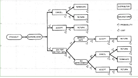
Using the classification rules we have proposed a new method of safety stock determination. This method uses the production flexibility as well as the ABCDEX classification of a product to determine a Cycle Service Level (CSL). The CSL denotes the chance of a stockout during the lead time. This CSL is then used to determine the amount of safety stock. The cycle stock follows from a production plan which is inputted into the model. Knowing the cycle- as well as safety stock, we can determine total stock, the expected number of stockouts and obsoletes. Knowing the expected number of stockouts, a stock availability is calculated. Knowing the total inventory, inventory costs can be calculated using a newly proposed formula. This formula includes costs of capital, internal relocations and external inventory costs. For the stockout- and obsolete costs we have also proposed formulas. These formulas are the result of decision trees which note all possible outcomes of an obsolete/stockout occurrence. We have then reduced these decision trees to a percentage of the products profit as final costs. This is 29% for obsolete costs and 35% for stockout costs.

Results

We have shown that we can improve the old way of determining safety stock. With approximately the same inventory and stock availability we can lower yearly total costs by more than 7%. We conclude that current levels of inventory and stock availability are close to optimal however, total costs can still be reduced by shifting safety stock between products. This leads to a decrease in both obsolete costs as well as stockout costs.

In short, we began this research with the aim of reducing inventory, however we conclude that this should not be pursued. Instead, the allocation of inventory to products should be optimized. This also means that harbour storage cannot be avoided but costs for this do not weigh up to the increase in stockout costs when lowering inventory.

Recommendations

We recommend Grolsch to start using the new type of safety stock determination and update it at least twice a year and preferably each quarter. Moreover, for the short term we advise Grolsch to look into the possibilities of dispatching from the harbour to reduce transport costs. Ideally, this is realized in the summer of 2018. For the medium term, we advise to create a business case for RFID tracking to

(7)

Glossary

Word or abbreviation

Meaning

CBS Central Bureau of Statistics

CO Changeover

COV Coefficient of variation

CSL Cycle Service Level

DoC Days of cover: the amount of forecasted sales that need to be covered by the inventory on hand.

FE Factory efficiency

FTE Full Time Equivalent

HL Hectoliters

KPI Key Performance Indicator

M&C Maintenance & Cleaning

ME Machine efficiency

MTD Month To Date

MTF Make To Forecast / Make to Stock

MTO Make To Order

NPD New Product Development

Off trade Groceries, retailers, etc

On trade Bars, restaurants, etc

Pal Pallets

SCP Supply Chain Planning

Shelf life The time a product is allowed to remain in inventory

SKU Stock Keeping Unit

SS Safety Stock

(10)

(11)

List of tables and figures

Figure 1.1. Brewing process

Figure 1.2. Warehouse layout Figure 1.4. External inventory Figure 1.6. Expected cost reduction

Figure 2.4. Root causes of stock increase in peak season Figure 2.5. Current inventory classification

Figure 2.6. Production throughput process.

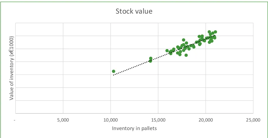
Figure 3.1. Decision tree for evaluating shortage costs (Oral et al, 1972) Figure 4.1. Correlation between inventory and value of inventory Figure 4.2. Correlation between inventory and weekly internal relocations Figure 4.3. QQ plot of total weekly inventory

Figure 4.4. Inventory costs of each root cause Figure 4.5. Decision tree for obsolete costs

Figure 4.6. Distribution of obsolete costs as percentage of profit Figure 4.7. Decision tree for stockout costs

Figure 4.8. Distribution of stockout costs as percentage of profit Figure 5.1. Production plan changes

Figure 6.1. Old and new classification comparison Figure 6.2. Production flexibility

Figure 6.3. Production flexibility of SKU 91135

Figure 6.4. Distribution of production flexibility over 2017 Figure 7.1. Safety stock model process

Figure 7.2. QQ plot of total weekly demand

Figure 9.1 Growth of breweries in the Netherlands (CBS) Table 2.1. Current inventory classification

Table 2.2. Pilot/Agile/Scale classification

Table 2.3. Example of opening days of cover during a week Table 3.1. Inventory control policies

Table 4.1. Chi-sqare test results

Table 4.2. Costs of empty shelf depending on the duration of the stockout Table 5.1. Production changes analysis line 4

Table 5.2. Production changes analysis line 7 Table 5.3. Production changes analysis line 8 Table 6.1. SKU changes from old to new classification Table 6.2. Pairwise comparison of supplier criteria Table 6.3. Results of supplier flexibility analysis Table 6.4. Pairwise comparison of flexibility criteria Table 6.5. Results of the MCA for the standard pilsner

Table 6.6. CSL per class for ABC and SCC combined classification Table 7.1. Chi-sqare test results

Table 7.2. Model output and actual values for 2017

Table 8.1. First model output using new method of safety stock determination Table 8.1. Improved model output using new method of safety stock determination Table 8.3. CSL matrix for optimal results

(12)

(13)

1. Introduction

In the framework of my study Industrial Engineering and Management at the University of Twente, I performed research at the Grolsche Bierbrouwerij Nederland B.V. (Grolsch). Here, I looked into inventory control and safety stock determination. Grolsch is a Dutch brewery that is a subsidiary of Asahi Group Holdings as of 2016. Grolsch not only produces the well-known brand Grolsch, they also produce brands such as Kornuit, De Klok, Amsterdam, Tyskie and Lech. The division of these beers is roughly 60 percent domestic over 40 percent export. Within the domestic market, on trade accounts for roughly 30 percent and 70 percent is off trade. This research is performed at the Supply Chain Planning (SCP) department in cooperation with the Finance, Warehouse and Demand Planning departments over the course of 6 months.

1.1. Supply Chain Planning department

The SCP department is responsible for the tactical planning and scheduling of the production lines and can be further divided into four sub departments.

1.1.1. Tactical planning

Tactical planning is done by two people who create a production plan for the coming 2 to 78 weeks. This plan is completely verified and updated once a week but is also continuously checked to accommodate any changes or uncertainties that have arisen. Naturally, the first weeks are rather fixed and the plan becomes more rough the further along they plan. Input for this plan consists of a demand forecast and production capacity. Besides this, they also need to take into account safety stocks, minimal batch sizes and maximum shelf lifes. Their output consists of a plan that shows how much beer of each Stock Keeping Unit (SKU) needs to be produced per week. This output is the input for the scheduling department.

1.1.2. Scheduling

(14)

INVENTORY CONTROL AT GROLSCH |Master thesis Kristian Kamp Page | 2

1.1.3. Brewing and filtration

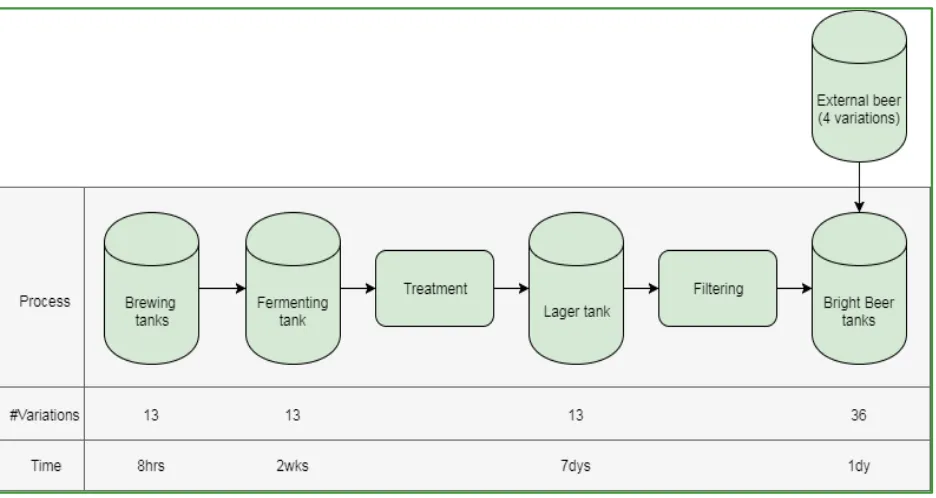
[image:14.612.75.543.156.405.2]

In order to accommodate the production plan on the lines, the person responsible for brewing and filtration needs to ensure that the beer is on time in a Bright Beer (BB) tank from where it can go to the production lines. Before the final beer is in a BB tank, several steps need to be taken that are displayed in Figure 1.1.

Figure 1.1. Brewing process

As can be seen from the figure, the total time needed to produce beer is approximately 3 weeks.

1.1.4. Material planning

(15)

1.2. Finance department

At Grolsch, a distinction is made between commercial finance and operations finance. Most relevant to this research are the people that make up the operations finance department. They create operational budgets and control whether the current expenses are in line with the budgets of this year. Moreover, they carefully monitor cost drivers and regularly report Key Performance Indicators (KPIs) such as fixed and variable production costs, beer losses, machine and factory efficiency and FTE’s to upper

management.

1.3. Demand planning department

Within demand planning, two persons are responsible for the creation of a demand forecast. This is done by analysing historical data of the last two to three years. This historical consumer data forms the baseline. Next, this baseline is corrected for changes in weather and, most important, promotions. Whereas a few years ago, a major client of Grolsch had approximately 12 promotions a year, this has increased to 16 per year. Given the fact that promotions are often only communicated a week in advance, the task of creating a reliable forecast has therefore become increasingly difficult.

1.4. Warehouse department

The warehouse department is responsible for storing all goods, both raw materials and finished

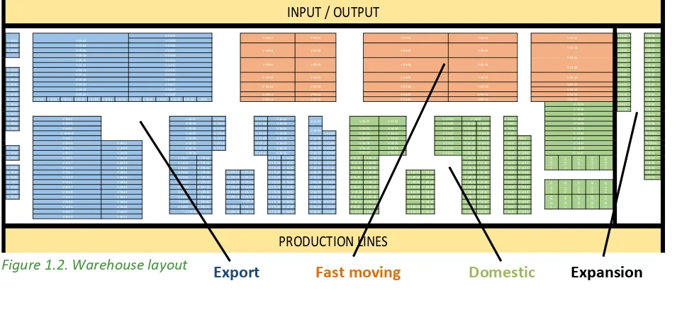
products, optimally. The warehouse for finished goods can hold a theoretical maximum of 22,376 pallets however, the practical limit lies around 19,500 because some moving space is required too. The

complete area for finished goods is displayed in Figure 1.2. The warehouse is split up into a fast moving

[image:15.612.71.552.457.693.2]

area, export area and domestic area. Lately, the practical limit of 19,500 pallets is more and more reached and exceeded causing the warehouse to use storage from locations that were originally not designated as finished goods storage, such as the green locations at the far right. Now that these areas begin reaching maximum capacity too, they resort to storage at the harbour in Enschede.

Figure 1.2. Warehouse layout

_Export

_{Fast moving}

_Domestic

_Expansion

L-03-00 L-03-02 L-03-01 L-03-04

V-05-03 L-03-03 L-03-06

V-05-05 L-03-05 L-03-08

L-03-07 L-03-10 L-03-09 L-03-12 L-03-11 L-03-14

V-05-09 L-03-13 L-03-16

V-05-11 L-03-15 L-03-18

V-05-13 L-03-17 L-03-20

V-05-15 L-03-19 L-03-22

V-05-17 L-03-21 L-03-24

V-05-19 L-03-23 L-03-26

V-05-21 V-10-65 V-10-63 V-10-61 V-10-59 V-10-57 V-10-55 V-10-53 V-10-51 V-10-49 V-10-47 V-10-45 V-10-43 V-10-41 L-03-25 L-03-28

V-05-23 L-03-27 L-03-30

V-05-25 L-03-29 L-03-32

V-05-27 L-03-34

V-19-02 V-17-02 V-17-01 V-13-01 L-03-36

V-19-04 V-17-04 V-17-03 V-13-04V-13-04 V-13-03 L-03-38

V-19-06 V-17-06 V-17-05 V-13-06V-13-06 V-13-05 L-03-40

V-17-08 V-17-07 V-15-02 V-13-08V-13-08 V-13-07 TP-03-01

V-17-10 V-17-09 V-16-05 V-15-04 V-13-10V-13-10 V-13-09 Pallets TP-03-02 V-17-12 V-17-11 V-16-07 V-15-06 V-13-12V-13-12 V-13-11 V-12-04 TP-03-03

V-19-08 V-17-14 V-17-13 V-16-09 V-15-08 V-13-14V-13-14 V-13-13 V-12-06 L-03-42

V-19-10 V-17-15 V-16-11 V-15-10 V-13-16V-13-16 V-13-15 V-12-08 L-03-44

V-19-12 V-17R-02 V-17L-01 V-16-18 V-16-13 V-15-12 V-15-15 V-14R-02 V-14L-01 V-13-18 V-13-17 V-12-10 L-03-46 V-17R-04 V-17L-03 V-16-20 V-16-15 V-15-14 V-15-17 V-14R-04 V-14L-03 V-13-20 V-13-19 V-12-12 L-03-48 V-19-14 V-17R-06 V-17L-05 V-16-22 V-16-17 V-15-16 V-15-19 V-14R-06 V-14L-05 V-13-22 V-13-21 V-12-14 L-03-50 V-19-16 V-17R-08 V-17R-01 V-17L-02 V-17L-07 V-16-24 V-16-19 V-15-18 V-15-21 V-14R-08 V-14R-01 V-14L-02 V-14L-07 V-13-24 V-13-23 V-12-16 L-03-52 V-19-20 V-17R-10 V-17R-03 V-17L-04 V-17L-09 V-16-26 V-16-21 V-15-20 V-15-23 V-14R-10 V-14R-03 V-14L-04 V-14L-09 V-13-26 V-13-25 V-12-18 L-03-54 V-19-22 V-17R-12 V-17R-05 V-17L-06 V-17L-11 V-16-28 V-16-23 V-15-22 V-15-25 V-14R-12 V-14R-05 V-14L-06 V-14L-11 V-13-28 V-13-27 V-12-20

V-19-24 V-17R-14 V-17R-07 V-17L-08 V-17L-13 V-16-30 V-16-25 V-15-24 V-15-27 V-14R-14 V-14R-07 V-14L-08 V-14L-13 V-13-30 V-13-29 V-12-22 V-19-26 V-17R-16 V-17R-09 V-17L-10 V-17L-15 V-16-32 V-16-27 V-15-26 V-15-29 V-14R-16 V-14R-09 V-14L-10 V-14L-15 V-13-32 V-13-31 V-12-24 V-19-28 V-17R-18 V-17R-11 V-17L-12 V-17L-17 V-16-34 V-16-29 V-15-28 V-15-31 V-14R-18 V-14R-11 V-14L-12 V-14L-17 V-13-34 V-13-33 V-12-26 V-17R-20 V-17L-19 V-16-36 V-16-31 V-15-30 V-15-33 V-14R-20 V-14L-14 V-14L-19 V-13-36 V-13-35 V-12-28 V-17R-22 V-17R-13 V-17L-16 V-17L-21 V-16-38 V-16-33 V-15-32 V-15-35 V-14R-22 V-14R-13 V-14L-16 V-14L-21 V-13-38 V-13-37 V-12-30 V-17R-15 V-17L-18 V-17L-23 V-16-40 V-16-35 V-15-34 V-15-37 V-14R-24 V-14R-15 V-14L-18 V-14L-23 V-13-40 V-13-39 V-12-32

V-02-01 V-02-02 V-04-03

V-05-01 V-05-02

V-04-01 V-04-02 V-03-01 V-03-02

V-02-05

V-05-12 V-04-13 V-02-08

V-05-14 V-04-15 V-05-06 V-04-07

V-05-08 V-04-09 V-02-06

V-05-10 V-04-11

V-04-06 V-03-05 V-03-06

V-02-10 V-05-18 V-04-19

V-05-20 V-04-21 V-04-10 V-03-09 V-03-10 V-02-09 V-02-12

V-05-16 V-04-17

V-04-08 V-03-07 V-03-08 V-02-07

V-04-14 V-03-13 V-03-14 V-02-13 V-02-18

V-12-01

V-05-22 V-04-23 V-02-14

V-05-24 V-04-25 V-04-12 V-03-11 V-03-12 V-02-11 V-02-16

V-13-02 V-12-07

V-19-03 V-18-03 V-16-04 V-14-03 V-12-09

V-12-03 V-12-05 V-19-01 V-18-01 V-16-02 V-16-01 V-15-01 V-14-02 V-14-01

V-19-06-A V-18-07 V-16-08 V-15-05 V-14-06

V-19-05 V-18-05 V-16-06 V-16-03 V-15-03

V-18-09 V-16-10 V-15-07 V-14-08 V-14-09

V-14-13 V-12-19

V-14-04 V-14-05 V-12-11

V-14-07 V-12-13

V-14-15 V-12-21

V-12-15

V-19-09 V-18-02 V-18-11 V-16-12 V-15-09 V-14-10 V-14-11 V-12-17

V-19-13 V-18-06 V-18-15 V-16-16 V-15-13 V-14-14 V-19-11 V-18-04 V-18-13 V-16-14 V-15-11 V-14-12 V-19-07

V-19-21 V-18-14 V-18-23 V-19-23 V-18-16 V-18-25

V

-1

2

-3

1

V-19-17 V-18-10 V-18-19 V-19-19 V-18-12 V-18-21 V-19-15 V-18-08 V-18-17

V -1 2 -2 3 V -1 2 -2 5 V -1 2 -2 7 V -1 2 -2 9 V-18-24 V-18-33 V -1 2 -4 3 V -1 2 -4 5 V -1 2 -4 7 V -1 2 -3 9 V -1 2 -4 1

V-19-27 V-18-20 V-18-29 V-19-29 V-18-22 V-18-31 V-19-25 V-18-18 V-18-27

V -1 2 -3 3 V -1 2 -3 5 V -1 2 -3 7 V-04-05 V-05-04

INPUT / OUTPUT

PRODUCTION LINES

V-19-37 V-18-30 V-17R-24 V-19-39 V-18-32 V-02-04 V-02-03 V-03-04 V-03-03 V-04-04 V -1 2 -4 9 V -1 2 -5 1

V-19-33 V-18-26 V-18-35 V-17L-14 V-19-35 V-18-28 V-18-37

(16)

1.5. Reason behind research

The practical limit for the warehouse at Grolsch lies around 19,500 pallets. In the past year, inventories have risen steadily and often exceeded this limit. On average, in 2017 inventory increased by 18% compared to 2016.

High levels of inventory are costly for several reasons. In Chapter 4 we will go into detail of all the costs which Grolsch faces when inventory rises. For now, we focus on one particular cost factor, namely external inventory costs.

(17)

[image:17.612.72.543.65.315.2]

Figure 1.4. External inventory

In order to estimate expected costs for the future we use the sales forecast for 2018. The amount of stock can also be described as the amount of forecasted sales in weeks that are covered with it. This cover varies from roughly 2 weeks up and till 3 weeks. In summer, sales are highest and thus this cover is small whereas in winter this cover is high. Also, in the period leading up to the summer, this cover is relatively high because of strategic stock build up. During peak periods, production capacity is not sufficient to keep up with demand. In order to prevent out of stocks, production is therefore scaled up before peak periods in anticipation of these high levels of sales. This is what is meant with strategic stock build up.

We assume that the number of weeks of forecasted sales that are covered with the inventory is highest at the start and end of the year and lowest in the middle of the year. To calculate this cover per week we choose to create a parabola equation as described in formula 1.1. The reason for choosing this particular equation is that its symmetrical, meaning that the first half of the year, the days of cover decreases similarly as how it increases the second half of the year. This corresponds to the data of the past two years.

#𝑤𝑒𝑒𝑘𝑠 𝑜𝑓 𝑓𝑜𝑟𝑒𝑐𝑎𝑠𝑡𝑒𝑑 𝑠𝑎𝑙𝑒𝑠 𝑐𝑜𝑣𝑒𝑟𝑒𝑑 𝑏𝑦 𝑠𝑡𝑜𝑐𝑘 = 𝑎(𝑥 − 26)

2

+ 𝑏

(1.1)

In formula 1.1, x denotes the week of the year, 26 describes week 26; the middle of the year, b will denote the lowest point and a will follow from substituting the highest point. Total forecasted sales for 2018 are similar to 2017. It is not expected to increase or decrease significantly, nor does it show significant shifts in peak or low periods. It is therefore safe to assume that the average inventory will remain the same as well if nothing else is done. If we use a value of 2.2 weeks for b; the minimum and a value of 3 weeks for the maximum, average inventory over 2018 amounts to 18,415 pallets, the same as for 2017.

500 1,000 1,500 2,000 2,500

18.2016 21.2016 24.2016 27.2016 30.2016 33.2016 36.2016 39.2016 42.2016 45.2016 48.2016 51.2016 02.2017 05.2017 08.2017 11.2017 14.2017 17.2017 20.2017 23.2017 26.2017 29.2017 32.2017 35.2017 38.2017 41.2017 44.201

7

47.2017 50.2017

Pa

lle

ts

Week

(18)

INVENTORY CONTROL AT GROLSCH |Master thesis Kristian Kamp Page | 6 The equation then becomes the following:

#𝑤𝑒𝑒𝑘𝑠 𝑜𝑓 𝑓𝑜𝑟𝑒𝑐𝑎𝑠𝑡𝑒𝑑 𝑠𝑎𝑙𝑒𝑠 𝑐𝑜𝑣𝑒𝑟𝑒𝑑 𝑏𝑦 𝑠𝑡𝑜𝑐𝑘 = 0.00133(𝑥 − 26)

2

_{+ 2.2}

_(1.2)

We assume that demand, and therefore stock level, is normally distributed with mean µ and standard deviation σ. From historic data we have also calculated the standard deviation.

Using the formula to calculate expected stockouts during a cycle we can also calculate the expected number of pallets that will exceed 19,500 given the expected stock level. We assume that this is the amount that will be stored in the harbour. Given the expected weekly stock level in the harbour we can calculate the required time and the amount of trucks needed for harbour transport to obtain expected costs. Detailed calculations of this can be found in Appendix I.

The expected total costs for external storage is approximately 85,000 euros for 2018. The reason that expected costs rise in 2018 is due to the fact that external storage was not used in the first 10 weeks of 2017 whereas this will be a realistic possibility in 2018 if no interventions take place.

When we are able to achieve a reduction in inventory, the first few pallets of reduction cause major savings whereas this effect reduces until harbour storage has become unnecessary and costs for external storage become zero. To illustrate this effect, we have made the same calculations for

(19)

[image:19.612.73.541.74.314.2]

Figure 1.6. Expected cost reduction

In this section, we have shown that if nothing is done, costs are expected to increase by 35,000 euros. If we can achieve a reduction of 1,000 pallets, we can ensure costs will remain the same for 2018. If we can achieve a reduction of 3,000pallets, we expect harbour storage to become redundant and savings on external inventory costs in 2018 will amount to 85,000euros. Besides this, other variable costs will decrease as well with every pallet that is reduced. This is further illustrated in Chapter 4.

€ -€ 10,000 € 20,000 € 30,000 € 40,000 € 50,000 € 60,000 € 70,000 € 80,000 € 90,000 € 100,000

- 1,000 2,000 3,000 4,000 5,000 6,000

Exp

ected

cos

ts

Reduction in pallets

(20)

1.6. Problem formulation

Over the past two years, Grolsch’ inventories have risen beyond the limits of the warehouse. When the maximum capacity of the warehouse is reached and exceeded, extra costs have to be made by storing goods in the harbour. Grolsch therefore wishes to optimize these inventories but at the same time service towards its customers and production efficiency may not drop below target levels.

1.7. Research goal and questions

Now that the problem is clearly defined, we can formulate our research goal:

To analyze past and present production planning decisions and to develop a tool that will determine optimal amounts of safety stock while maintaining target service levels.

To achieve this goal, the following research questions are used: 1. Current situation

1.1.What has caused Grolsch’ inventories to rise?

1.2.What does Grolsch’ current ABC inventory classification look like? 1.3.What inventory control policies are used at Grolsch?

1.4.How are inventory control parameters determined at Grolsch? 2. Literature

2.1.How can inventory be classified?

2.2.Which types of inventory control policies are described in literature 2.3.What is the relation between safety stock and finance?

2.4.What is the relation between safety stock and customer service? 3. Model formulation and development

3.1.What requirements and constraints are there for an inventory model? 3.2.How can we improve the current inventory control methods?

3.3.How do we ensure the validity of a new model? 4. Model implementation and evaluation

4.1.What are costs and service levels associated with the new model and how does this score compared to the old methods?

(21)

1.8. Scope and limitations

The amount of inventory that ends up in the warehouse is a factor of many different things. In the scope of this research it is not possible to investigate all these factors. Our research deals with Finished Goods (FG) inventory. The brewing process will not be investigated as it is working around 60% capacity and has seldom been a reason for production issues. Also, storage for raw materials is merely a fraction of the total warehouse and shall therefore not be further looked into. In addition, Grolsch produces both on a Make to Order (MTO) as well as a Make to Forecast (MTF) system. In literature, the MTF system is better known as Make to Stock. Because the demand for MTO products is known and fixed, safety stock is not needed for these products and all MTO products will not be taken into consideration. Next, within the scope of this research, forecasting techniques will not be researched. Forecasting is done by the Demand Planning department that uses sophisticated tools. It will be very time consuming to fully comprehend the techniques used in these tools and it is expected that optimization of them will not lead to significant improvements. Finally, this research will focus mainly on safety stock. Recently, optimal production batches and frequencies (and with it cycle stock) have been researched in depth and will not likely be changed again. We will analyze these decisions with regards to inventory consequences but we will not try to optimize these parameters again.

1.9. Deliverable

The final deliverable to Grolsch will be twofold. First of all, this research will provide a cost analysis of production planning decisions that are made in the past. This research aims to uncover the savings as well as the expenses that have been realized by the decisions of the SCP department.

(22)

1.10. Method and planning

As stated before, this research will be conducted over the course of six months. It is therefore vital to plan this time well. In this section you find the method that is used to answer each research question. 1. Current situation

1.1. What has caused Grolsch’ inventories to rise?

First of all, we will interview warehouse managers and production planners to gain insights into the root causes of Grolsch’ rising inventories. The result of this will be a list of possible root causes. Next, we will analyse historical data to determine whether each possible cause has attributed to the rising inventory as well as the degree in which they have done so. This is done in Section 2.1.

1.2.What does Grolsch’ current ABC inventory classification look like?

The current ABC classification has been made by the people from the Demand Planning and Sales departments. Many products however, are unclassified. We will therefore uncover which products are classified and why, as well as the grounds for determining a products classification. Moreover, we will calculate, among other things, the percentage of items and revenues belonging to each classification in order to determine whether Grolsch’ classification is in line with current practices. This is done in Section 2.2.

1.3.What inventory control policies are used at Grolsch?

The SCP department uses several tools to determine the levels of safety stock for each SKU. We will study the workings of these tools to uncover the underlying calculations and uncover what it does and does not take into account. This is done in Section 2.3.

1.4.How are inventory control parameters determined at Grolsch?

This research question will also be answered by interviewing the people from the SCP department. In the recent past they have performed research on optimal production batches and frequencies and therefore know exactly which parameters have influenced their decisions and how they are determined. This is done in Section 2.3.

2. Literature

2.1. How can inventory be classified?

All common ways of inventory classification will be researched in literature and an overview of their advantages and disadvantages will be made. With this we hope to find the method that is most suitable for Grolsch. This is done in Section 3.1 as well as Chapter 6.

2.2. Which types of inventory control policies are described in literature

Similar to inventory classification, many different kinds of inventory control policies exist in

literature. We will investigate which policy is most similar to Grolsch’ current practices and research its advantages as well as disadvantages. This is done in Section 3.2.

2.3. What is the relation between safety stock and customer service?

(23)

2.4. What is the relation between safety stock and finance?

By researching literature that approaches inventory from a financial perspective, we hope to find knowledge to help us in determining optimal amounts of safety stock to create the balance between costs of high levels of inventory and costs of stockouts due to too little inventory. This is done in Section 3.4.

3. Production planning decisions

3.1.What are the effects of the historic production planning decisions?

In the beginning of 2017, production plans for line 4 and 7 have been changed. By comparing data from before and after this implementation we hope to determine the changes in efficiency as well as savings and costs which this has caused. With this analysis, we hope to determine whether or not these production planning decisions have caused savings and were thus justified. This is done in Chapter 5.

4. Model formulation and development

4.1.How can we evaluate different levels of safety stock?

In order to determine the optimal amounts of safety stock, we need ways of evaluating safety stock. We will propose formulas of evaluating inventory, stockouts and obsoletes to be able to calculate total expected costs corresponding to a level of safety stock per product. We will do this by

combining methods from literature and input from experienced managers. This is done in Chapter 4. 4.2. What requirements and constraints are there for an inventory model?

By studying the current tools as well as by interviewing all users of the current model, we hope to uncover all requirements it should meet and constraints it should incorporate. By ways of

prototyping we can let users try out a new model which will then most likely result in feedback as to what is missing. This is done in Section 7.1.

4.3. How can we improve the current inventory control methods?

When it is known how the current tools work, we will study literature on safety stock determination to determine which method comes closest to practice. We will then analyse alternatives and see what options we have to improve the current inventory model. From each option we will analyse its advantages and disadvantages and finally choose the best among them. This is done in Section 7.2. 4.4.How do we ensure the validity of a new model?

First of all, we will try to enclose the current model in certain rules and inventory control policies to be able to simulate the current way of safety stock determination. This simulation will be run on historical data to check whether the result of the simulation is in line with the actual levels of stock and associated costs. When we have made sure this simulation is a reliable representation of the truth we have ensured the validity of the model. We can then change certain input parameters such as the Days of Cover to create a valid new model. This is done in Section 7.3.

5. Model implementation and evaluation

5.1.What are costs and service levels associated with the new model and how does this score compared to the old methods?

From research question 2.3 and 2.4 we will have equations in determining costs and service levels from certain input parameters. With this, we can easily calculate costs and service levels from both old as well as new models. This is done in Section 8.1.

5.2. What is the effect of marginally increasing/decreasing target service levels?

(24)

(25)

2. Current situation

The following chapter provides information on the current practices at Grolsch. We start in Section 2.1. with a root cause analysis to find out why Grolsch’ inventories have risen in comparison to 2016 or why they may be high in general to answer research question 1.1. Next, we research Grolsch’ current ABC classification to provide an answer to research question 1.2. Finally, we analyze the current inventory control methods and safety factor determination in Section 2.3 to answer research question 1.3 and 1.4.

2.1. Root cause analysis

As was shown in Chapter 1, average inventory for 2017 was 18,415. The historic deviation of the inventory level is 1,679 pallets which means that there have been peaks where inventory has reached and exceeded the practical limit of 19.500. Not surprisingly, these peaks occurred in peak season. Due to this, external storage in the harbour was needed at that time. Before we can try to reduce Grolsch’ inventories it is paramount to uncover what has caused Grolsch’ inventories to rise. To do so, we compare the peak season of 2017 with the peak season of 2016. We chose to compare peak season and not the whole year because it is during this time that increased inventory really matters. An increase in inventory at this time means that the limits of the warehouse may be reached and exceeded and external inventory costs are made. We define peak season to range from week 14 up and till week 39. Average inventory in 2016 was 15,254 pallets during this time and in 2017 this was 19,087. This is an increase of 3,833 pallets or 25%. To uncover the root causes behind this increase we have started by interviewing managers of the SCP department, warehouse department and demand planning

department. In addition, we have explored possible root causes from literature and practice as well. The possible root causes that have resulted from this can be categorized as follows:

1. Too much cycle stock

1.1. Caused by increased sales 1.1.1. Increased sales overall

1.1.2. Shift of sales from low season to peak season

1.2. Caused by adding new products (NPDs) faster than delisting old ones 1.3. Caused by not selling all which was forecasted

1.4. Caused by producing more than was planned 1.5. Caused by producing in larger batches 2. Too much safety stock

2.1. Caused by a faulty classification

(26)

2.1.1. Too much safety stock

Safety stock is determined by means of a Days of Cover (DoC) criterion. How this works exactly will be explained in Section 2.3. This parameter is partly based on the ABC classification of a product. This classification has not been updated in the last two years. It can therefore not explain a rise in inventory but it may be a reason why inventory is too high in general. With an inaccurate and outdated

classification, safety stock is placed at the wrong products. Also, when too many products are marked as important, safety stock is unnecessarily high. Section 2.2.will provide more information on Grolsch’ current ABC classification and Chapter 5 will deal with updating Grolsch’ classification.

2.1.2. Increased sales

Perhaps the most logical explanation would be an increase in sales. Naturally, when sales systematically increase, stock increases accordingly. We make the distinction between an overall increase in sales and the shift of sales from low to peak season. In the latter case, sales may not have increased throughout the year but it has shifted to peak season.

Overall sales increase

(27)

Increased sales in peak season

The fact that sales of beer are higher in summer than in winter is not surprising and has always been the case. However, in 2017 this difference has become greater.

It is clearly visible that in 2017 the peak in summer is higher and the lowest point in winter is lower compared to 2016. In short, the past year, sales have shifted more towards high season. In fact, this is not an isolated event of the past year but experts within Grolsch confirm that this trend has been happening for a while.

To illustrate this seasonality shift we can calculate that in 2016, 13% of annual sales was sold in the time period ranging from week 1 up and till week 8. 17% was sold in the time period ranging from week 21 up and till week 28. In 2017, this shifted to 11% and 20% respectively.

Naturally, the higher levels of sales in peak season still need to be produced however, there are certain limits to production that are very costly to increase. A solution is therefore to make use of strategic stock build up. This means that before peak periods, production is scaled up in anticipation of these high sales. Due to capacity constraints as well as obsolete risks, production cannot be brought forward too much. It is for these reasons that the trend of greater differences between low and high season causes extra planning challenges and increased levels of stock during high season as well as some weeks in advance.

During this time, inventory may have to be stored in the harbour causing extra costs, whereas in winter, savings are not significant due to the fact that there is always a minimum number of personnel and thus costs. Moreover, when sales shift towards a peak, variation increases which causes the predictability of sales to decrease. This causes a less accurate forecasting which may result in higher safety stocks or more stockouts.

In 2016, on average 7,695 pallets were sold weekly in peak season. In 2017, this was 8,320 pallets. This is an increase of 625 pallets weekly. Using formula 1.2 we can calculate the average number of weeks that are covered by the stock during peak season. This is 2.3 weeks.

(28)

2.1.3. NPD/Delisting

As is the case with any company manufacturing products, over time some products are added and some products are discontinued. At Grolsch, new products are called New Product Development (NPD) and when discontinuing a product, we speak of delisting a product. Another part of the explanation for a rise in inventory, is that the stock of NPDs grows faster than the stock of delisted products shrinks.

In peak season of 2017, 17 SKUs were newly added to the portfolio and 23 were delisted. However, the stock of the NPDs amounted to 758 pallets weekly whereas the stock of delisted products was only 545 pallets.

This difference of 213pallets is 6% of total stock increase.

2.1.4. Forecast bias

We define forecast bias to be the actual sales minus the forecasted sales. When sales are higher than forecasted, the warehouse is drained and inventory decreases. Especially when this happens a few weeks in a row, the effect on the warehouse can become quite significant. This has occasionally happened in 2016 whereas in 2017 this has not happened as often.

Unfortunately, no accurate historic forecast can be retrieved for export products but we assume these products have little effect on total forecast bias.

We conclude that in peak season of 2016, sales were systematically under forecasted whereas in 2017 sales were over forecasted. This means that in peak season of 2016, inventories have decreased due to unexpected sales whereas in 2017, products have remained on stock because forecasted sales did not occur.

(29)

2.1.5. Production error

We define production error to be the actual production minus planned production. When production is lower than planned, less products end up on stock and inventory decreases. This is what regularly happened in 2016 whereas it happened less in 2017. Naturally, deviating from a plan is not desirable and can cause, among other negative aspects, a higher risk of stockouts because products are not ready when expected. The fact that this error shows a relative increase is therefore actually a positive thing and should not be reverted. It has however, caused a stock increase of 714 pallets.

We conclude that production error has improved in the past year. This means that in 2017 there was a better adherence to the production plan causing more planned products to actually end up on stock than in 2016. Even though it has caused a stock increase, the fact that this error has improved in 2017 is therefore actually beneficial.

We do note however; it has been cause for a relative stock increase of 714 pallets which is 19% of total stock increase.

2.1.6. Batch size

When batch sizes increase, stock will increase by half of the batch size. For example, when producing 100 pallets per week, stock decreases from 100 to 0 and stock is therefore 50 pallets on average. When doubling this batch size to 200 pallets, average stock will be 100 pallets regardless of production

frequency. Early last year, the SCP department has critically reviewed its planning for production lines 4, and 7. This has changed several things in their planning, one of which is an increased average batch size. They have done so in order to achieve higher production efficiencies.

We compare the new and old plans for production lines 4 and 7. Total volume in the old and new situation is equal and it does not include any NPDs or delisted products. Changes between them can therefore fully be attributed to increased batch sizes.

For line 4, batch sizes have increased by 24% on average. This has caused a stock increase of 505 pallets. For line 7, batch sizes have increase by 3% on average. This has caused a stock increase of 118 pallets. The production plan of line 8 has also been reviewed and changed. The stock increase of this cannot be calculated exactly however, because a precise old and new plan does not exist. We could check the difference in planned batch size but it will also include the effects of sales increase, forecast accuracy and production error.

We conclude that stock increase due to larger batch sizes on line 4 and line 7 is 623 pallets. This corresponds to 16% of total stock increase.

(30)

(31)

2.1.7. Conclusion

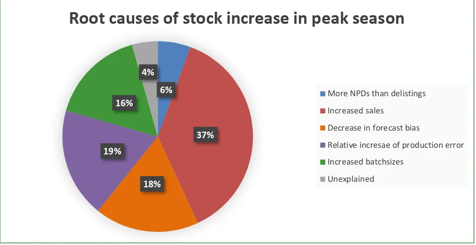
[image:31.612.72.542.130.372.2]

We have determined the degree in which each root cause has contributed to stock increase during peak season. This is summarized in Figure 2.4.

Figure 2.4. Root causes of stock increase in peak season

The smallest root cause is due to the fact that more NPDs have been added to the portfolio than have been removed from it. Today’s market is more demanding than ever and asks for high varieties, fast response to changes and being highly innovative. Introducing new products often is therefore key to survival and may be worth some extra inventory. Also, the forecast bias is not shockingly large and will be impossible to reduce completely as we are living in a stochastic world. Our focus will therefore not lie on these two aspects however; we will discuss them a little further in Chapter 9.

Next, we have seen that the reduced production error is in fact favorable and should not be changed. The increase in sales during peak season has the most significant effect. Unfortunately, we cannot influence when customers buy products (at least not within the scope of this research). This cause will therefore not be a part of further research.

This leaves us with one major root cause that can be influenced, which is batch size. As said before, the SCP has made some major changes to this last year and will therefore not easily revert their decisions. Therefore, we do not go into detail of optimal batch sizes and production frequencies. We will however, check whether the benefits of these changes were achieved and whether or not they weigh up to the increase in inventory. This will be done in Chapter 5.

Besides the root causes for rising inventory we suspect that inventory may be too high in general due to inaccurate classification of SKUs and therefore inaccurate placement of safety stock. This will be further researched in the next section as well as Chapter 6.

6%

37%

18% 19%

16% 4%

Root causes of stock increase in peak season

More NPDs than delistings Increased sales

Decrease in forecast bias

Relative incresae of production error Increased batchsizes

(32)

2.2. ABC classification

Grolsch uses an ABC classification to distinguish between the importance of its products.

This classification is based on sales data but heavily supplemented by experience and insights from the people of the Demand Planning and Sales departments. It is not precisely known when this classification was completely revised and updated last but it is estimated that this was about two years ago. Contrary to what the name suggests, there are actually five classes in the ABC classification at Grolsch:

A. Products that are most important to Grolsch. B. Products that are fairly important to Grolsch. C. Products that are less important to Grolsch. D. Products that are produced on a MTO basis. X. Unclassified products.

The division of products in 2017 is shown in Table 2.1.

Classification #SKUs

Average stock '17 (pal)

Profits '17 (x1000€)

A 13% 39% 53%

B 8% 5% 3%

C 3% 1% 1%

D 8% 3% 2%

X 67% 52% 40%

Total 100% 100% 100%

Table 2.1. Current inventory classification

As can be seen in Table 2.1, 2/3rds of products are unclassified which take up more than half of the warehouse. These unclassified products are mainly (84%) export products and NPDs. Export products are sold by means of a transfer price which means their margin is low. Also, orders for export products arrive some weeks in advance, are therefore more predictable and require less safety stock. It would therefore not be accurate to classify them along with domestic products in the same way. NPDs are new products of which it is not yet known how they should be classified. However, given the fact that the classification has not been updated in a while, it is likely that some of these NPDs have matured and could now be given a classification. This will help in reducing overall inventory because most NPDs receive high levels of safety stock similar to class A products. This is because when introducing new products, stockouts are highly undesirable. It is highly likely, that many of these NPDs have now matured and may not contribute to profits as much to receive an A classification.

As can also be seen in Table 2.1, the majority of classified products are classified as A; most important. This is not in line with theory and the classic 80/20 rule of Pareto. This rule states that class A products should be a select few, usually around 20 percent, that cause 80 percent of the revenues. Instead, there are more A products than B and C combined while their revenues are nowhere close to 80%.

(33)

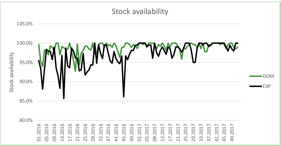
In fact, the Year to Date (YTD) SA for the domestic market is at 99.4% while the target lies at 98.3%. For the export market this is 98.9% compared to a target of 97.5%.

Figure 2.5. Current inventory classification

It can be argued that a significant amount of current class A products may actually be classified as B or C, resulting in less safety stock. This may reduce stock availability but the gap of more than 1% between the actual levels and the targets gives us some latitude. This will be examined in Chapter 6.

Next to the ABC classification, there exists another strategic classification at Grolsch. In this classification products may receive any of the following three classifications:

 Pilot: Products with annual sales less than 1,500HL

 Agile: Products with annual sales more than 1,500HL but less than 10,000HL

 Scale: Products with annual sales over 10,000HL The division for this classification can be found in Table 2.2.

Classification

#SKUs

Average stock '17 (pal) Profits '17 (x1000€)

Scale 24% 74% 83%

Agile 40% 22% 16%

Pilot 36% 4% 2%

[image:33.612.72.541.110.355.2]

Total 100% 100% 100%

Table 2.2. Pilot/Agile/Scale classification

This classification is more in line with the theory and the classic 80/20 rule but it is not used to determine safety stock of products so it has no effect on our level of inventory. Moreover, both classification methods are based only on sales and do not take into account production parameters or inventory holding costs.

80.0% 85.0% 90.0% 95.0% 100.0% 105.0%

01.2016 05.2016 09.2016 13.2016 17.2016 21.2016 25.2016 29.2016 33.2016 37.2016 41.201

6

45.2016 49.2016 01.2017 05.2017 09.2017 13.2017 17.2017 21.2017 25.2017 29.2017 33.2017 37.2017 41.2017 45.2017 49.2017

(34)

2.3. Inventory control policy and safety factor determination

As said in Chapter 1, the people from tactical planning create a production plan for the coming 2 to 78 weeks. This plan is completely updated once a week but is regularly changed throughout the week as well to accommodate any unexpected sales or production changes. Production is planned by means of a minimal Days of Cover (DoC) criterion. This parameter describes the minimal number of days of

forecasted demand that needs to be covered by on-hand inventory at the end of the week. As soon as inventory is expected to drop below this criterion, production will be planned in that specific week or before so this does not happen. Grolsch therefore uses a Reorder Point (ROP) that is determined by the DoC criterion. Because in theory the inventory is checked once a week, Grolsch’ inventory control policy has most similarities to a (R,s,S) system. This means that with an interval of R, in our case 1 week, it is checked whether inventory is below a certain point s, in our case described by the DoC criterion. If this is the case, an amount will be ordered/produced such that total inventory is raised to a level S again. In our case, this level S is not composed of a certain amount of pallets but rather determined in such a way that the DoC for that particular product is not excessively large nor is it below the criterion that is set. In this section we start by explaining the relation between this DoC parameter and safety stock. Subsequently, we explain Grolsch’ way of measuring service towards the customer and finally, we discuss production batch sizes and frequencies.

2.3.1. Days of cover and safety stock

Production at Grolsch runs mostly from Monday to Friday. We assume that production is finished at the end of the day and the chance that production is planned on a specific day is equal for every day. In other words, production lead time is uniformly distributed with possible values from 1 to 5 and equal probabilities 0.2. The expected production lead time is simply the average of the possible values; in our case 3 days. The DoC parameter includes this expected production lead time as well as some safety buffer. If a certain product has a minimal DoC of 5 days, it means that at the end of the week, inventory should be sufficient to cover the next 5 working days. 3 of these days is expected production lead time which can be considered as cycle stock. This leaves us with 2 days of safety stock. In other words, safety stock at Grolsch is the DoC minus 3 days, multiplied by the forecasted daily demand. To simplify our calculations slightly, we approximate safety stock using the average weekly demand denoted by µ instead of the forecasted daily demand. Naturally, the DoC criterion is also converted to weeks by dividing it by 7 days. This is shown in formula 2.1.

SafetyStock =

DoC−3

7

∗ µ

(2.1)

DoC: Days of Cover µ: Weekly demand

(35)

2.3.2. Stock availability and Ready Rate

To measure service towards its customer, Grolsch uses the KPI stock availability. Each morning, the people from the tactical planning department check the amount of products that have sufficient inventory to cover demand for that day. This percentage of total products is listed as the stock

availability (SA) for that day. The SA over a certain time period is simply the average SA of all days within that time period. This is similar to what in the literature is described as a Ready Rate. The ready rate describes the fraction of time during which stock is positive. To give an example, suppose opening days of cover for a certain week is as described in Table 2.3.

Monday

Tuesday

Wednesday

Thursday

Friday

Ready

Rate

Product 1 5.51 0.90 2.37 3.71 2.73 80%

Product 2 2.25 6.41 7.64 2.54 9.94 100%

Product 3 9.46 0.53 0.10 5.30 3.85 60%

Product 4 4.57 4.64 3.89 5.50 6.88 100%

Stock Availability

100% 50% 75% 100% 100% 85%

Table 2.3. Example of opening days of cover during a week

When at the beginning of the day, the DoC for a product is smaller than 1 it means the demand for that day cannot be met in full with the on hand inventory. These occasions are marked in red. SA for each day is defined as the number of products with sufficient stock divided by the total number of products. Total SA is the average over all days and amounts to 85%. The Ready Rate lists the fraction of time that each product has sufficient stock. This is determined for each product and the average over all products amounts to 85% as well. Let us denote xij as follows:

𝑥

𝑖𝑗

= {

0 𝑖𝑓 𝐷𝑜𝐶 < 1 𝑓𝑜𝑟 𝑝𝑟𝑜𝑑𝑢𝑐𝑡 𝑖 𝑜𝑛 𝑑𝑎𝑦 𝑗

1 𝑖𝑓 𝐷𝑜𝐶 ≥ 1 𝑓𝑜𝑟 𝑝𝑟𝑜𝑑𝑢𝑐𝑡 𝑖 𝑜𝑛 𝑑𝑎𝑦 𝑗

(2.2)

Let the number of products range from i=1 to n and the number of days from j=1 to m. It follows that Stock Availability is defined as follows:

SA =

1

𝑚

∗ ∑

(

1

𝑛

∗ ∑

𝑥

𝑖𝑗

)

𝑛 𝑖=1 𝑚

𝑗=1

(2.3)

The ready rate is defined as follows:

Ready Rate =

1

𝑛

∗ ∑

(

1

𝑚

∗ ∑

𝑥

𝑖𝑗

)

𝑚 𝑗=1 𝑛

𝑖=1

(2.4)

It can easily be seen that both equations can be rewritten to the following:

Stock availability = Ready Rate =

1

n

∗

1

m

∗ ∑

∑

x

ij m j=1 n

(36)

2.3.3. Production batch sizes and frequencies

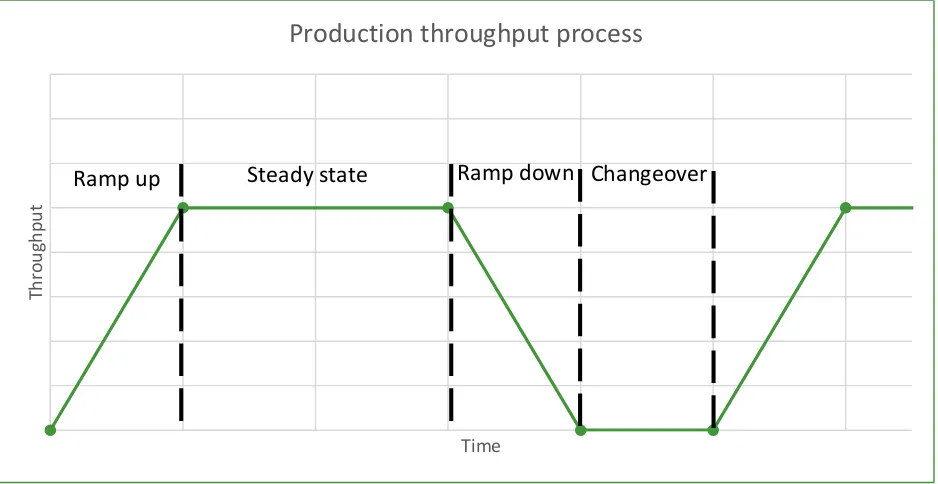
Production is always done in batches. For each batch there is a certain time period that is needed before everything is running smoothly at full capacity. We define this as the ramp-up. After this time

[image:36.612.73.542.175.417.2]

production runs in a so called steady-state. Production is concluded by a ramp-down meaning that production slowly comes to a halt. After this, the next product may be produced so a changeover takes place. This is illustrated in Figure 2.6.

Figure 2.6. Production throughput process.

Machine efficiency is greatest during the steady-state. As was said before, the SCP has recently made changes to production plans for line 4, 7 and 8. The main reasons for doing this is to reduce changeover time and increase the steady-state time causing greater machine efficiency. As has already been proven in Section 2.1, a downside of this is that is has caused inventories for these products to rise. In Chapter 5, we will investigate whether the benefits of efficiency outweigh the drawback of risen inventories. Finally, at Grolsch, certain products need to be grouped into families for production reasons. Changing one SKUs frequency therefore results in a need to change other SKUs frequencies too. This causes the optimal EOQ calculations to become quite complex. In the past year, extensive research has been done at Grolsch to determine the optimal production frequencies given these restrictions. We therefore assume that the results of this are (near) optimal and treat these frequencies per SKU as fixed input.

Th

ro

u

gh

p

u

t

Time

Production throughput process

(37)

2.4. Conclusion

In this chapter it has been shown that the major root cause for Grolsch’ risen inventories is increased sales during peak season. Precisely because most inventory costs are incurred during this time, this root cause is quite significant. Unfortunately, we cannot influence when customers buy our product (at least not within the scope of this research) so little can be done about this root cause.

We have also shown that recently it has been decided to increase batch sizes for certain products to achieve greater production efficiencies and that this has caused stock to increase as well. In Chapter 4 we research if these greater efficiencies have indeed been achieved and if they weigh up to the drawback of increased inventory.

In Section 2.2 we have shown that Grolsch’ current ABC classification has too many products marked as A. This may be a reason for too high levels of safety stock and therefore we will update this classification in Chapter 6 in order to achieve a reduction in safety stock.

(38)

(39)

3. Literature review

Before we can research improvements for Grolsch’ inventory classification and safety stock determination, it is vital to comprehend all theory behind it. In this chapter, all relevant theory of inventory classification and control is researched. We start by exploring all kinds of inventory

classification methods in Section 3.1 to answer research question 2.1. In Section 3.2 and 3.3 we explore the relation between customer service, finance and safety stock to answer research questions 2.3 and 2.4. Finally, Section 3.4. deals with different kinds of inventory control policies and the corresponding ways of determining safety stock. This will provide an answer for research question 2.2.

3.1. Inventory classification

One commonly used technique for classifying inventory is by means of an ABC analysis. This analysis, sometimes also called Pareto analysis, is partly based on the law of Italian economist Vilfredo Pareto who observed that 20 percent of the Italian population owned 80 percent of the land (Pareto, 1935).For inventory classification, classical ABC analysis says that roughly 20 percent of the products account for 80 percent of the annual dollar usage. The SKUs in this group will get an A classification. The next group, having a B classification, are roughly the next 30 percent of items that account for 15 percent of annual dollar usage. The remainder, 50 percent of products accounting for only 5 percent of annual dollar usage, receive a C classification.

Next, most methods describe a fixed service level per class. Arguments for which class should receive the highest service level vary. Armstrong (1985) argues that A items should have the highest service levels because availability of these items is paramount. For C items he says that stockouts should be risked so that they can earn a reasonable rate of return. On the other hand, Knod and Schonberger (2001) claim that for C items it is not worth the effort to deal with stockouts and they should therefore receive the highest service level. (Teunter, Babai & Syntetos, 2010).

This traditional ABC analysis is only influenced by the costs and sales of the product. Extensions and adaptations of this analysis are widely researched and include other criteria such as revenues or profits (Silver, Pyke & Thomas, 2016), lead time and criticality (Chen, 2008), and availability and commonality (Flores & Whybark, 1987). Moreover, classification need not be restricted to single criteria or three classes (Ultsch, 2002). According to Graham (1987), multiple classes are often used but are usually limited to six at the most. Also, a number of authors argue for the use of multiple criteria and use methodologies such as Weighted Linear Programming (Ramanathan, 2006; Zhou & Fan, 2007), AHP (Flores, Olson & Dorai, 1992) and Fuzzy classification (Chu, Liang & Liao, 2008).

(40)

INVENTORY CONTROL AT GROLSCH |Master thesis Kristian Kamp Page | 28 Subsequently, in their paper, Teunter, Babai & Syntetos (2010) propose a new cost criterion for ABC analysis in combination with fixed cycle service levels per class. This method takes criticality into account and they proof that it outperforms traditional ABC analysis as well as the method from Zhang et al.

They rank SKUs by the criterion of 𝑏∗𝐷

ℎ∗𝑄

where b stand for the shortage cost, D describes the demand

volume, h the holding cost and Q the order size. Next, they show that class A should be the first 20% of this criterion with the highest service level. Class B should be the next 30% and class C the last 50% with decreasing service levels. Their results show that this method results in almost half the safety stock costs compared to traditional demand value and demand volume criteria. (Teunter, Babai & Syntetos, 2010).

3.2. Inventory control and cycle stock

Inventory control has a direct relation with ordering quantities. Harris (1913) was the first to present a formula for optimal production ordering quantities. This formula is denoted below.

𝑄

∗

_{= √}

2𝐷𝐾

ℎ

(3.1)

D: Annual demand

K: Fixed costs per order or setup h: Annual holding costs per unit Q*: Optimal order quantity

The formula follows logically from the fact that total costs are calculated as follows:

𝑇𝐶 =

𝐷𝐾

𝑄

+

ℎ𝑄

2

+ 𝑃𝐷

(3.2)

D: Annual demand

K: Fixed costs per order or setup h: Annual holding costs per unit P: Purchase price per unit Q: Ordering quantity TC: Total costs

Other than ordering this fixed quantity Q, we can also choose to have a variable lot size. In this case, rather than ordering a fixed amount, we order as much as needed to raise inventory to a fixed level. In both cases we again have two choices. We can either review our inventory status periodically or continuously (Silver et al, 2016). This can be summarized by Table 3.1.

Periodic review

Continuous review

Fixed lot size (R,s,Q) (s,Q)

[image:40.612.67.547.655.708.2]

Variable lot size (R,s,S) or (R,S) (s,S)

Inventory control at Grolsch : a master thesis which analyzes inventory control at Grolsch and proposes a model to determine optimal levels of safety stock