Bayesian structural inference with applications in social science

(1)

A Thesis Submitted for the Degree of PhD at the University of Warwick

Permanent WRAP URL:

http://wrap.warwick.ac.uk/78778

Copyright and reuse:

This thesis is made available online and is protected by original copyright.

Please scroll down to view the document itself.

Please refer to the repository record for this item for information to help you to cite it.

Our policy information is available from the repository home page.

(2)

AUTHOR:Robert J. B. Goudie DEGREE:Ph.D.

TITLE:Bayesian structural inference with applications in social science

DATE OF DEPOSIT: . . . .

I agree that this thesis shall be available in accordance with the regulations governing the University of Warwick theses.

I agree that the summary of this thesis may be submitted for publication.

Iagreethat the thesis may be photocopied (single copies for study purposes only).

Theses with no restriction on photocopying will also be made available to the British Library for microfilming. The British Library may supply copies to individuals or libraries. subject to a statement from them that the copy is supplied for non-publishing purposes. All copies supplied by the British Library will carry the following statement:

“Attention is drawn to the fact that the copyright of this thesis rests with its author. This copy of the thesis has been supplied on the condition that anyone who consults it is understood to recognise that its copyright rests with its author and that no quotation from the thesis and no information derived from it may be published without the author’s written consent.”

AUTHOR’S SIGNATURE: . . . .

USER’S DECLARATION

1. I undertake not to quote or make use of any information from this thesis without making acknowledgement to the author.

2. I further undertake to allow no-one else to use this thesis while it is in my care.

DATE SIGNATURE ADDRESS

. . . .

(3)

M A E

G NS

I T A T MOLEM

U N

IV

ER

SITAS WARWICEN

SIS

Bayesian structural inference with applications in

social science

by

Robert J. B. Goudie

Thesis

Submitted to the University of Warwick

for the degree of

Doctor of Philosophy

Department of Statistics

School of Health and Social Studies

(4)

List of Tables

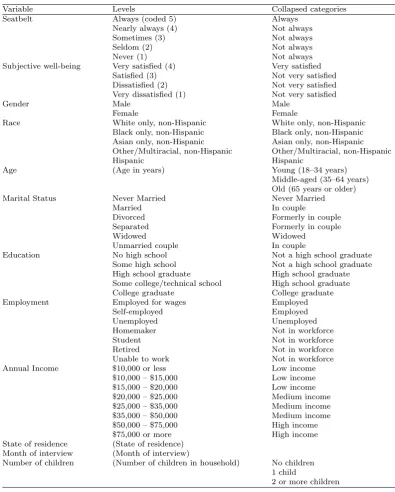
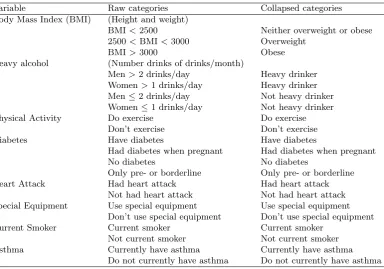
3.1 The main covariates used from BRFSS in Chapter 3. . . 59

3.2 Additional covariates from BRFSS used in model selection analyses in Chapter 3. . . 71

3.3 Questions used in the study from BRFSS in Chapter 3. . . 72

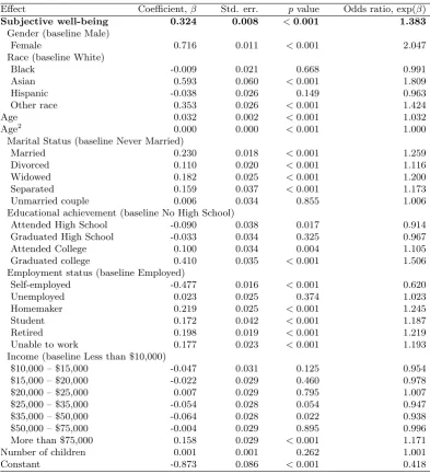
3.4 Logistic regression equations for seatbelt use. . . 73

3.5 Ordinary Least Squares (OLS) equations for seatbelt use. . . 74

5.1 Structural Hamming distances (SHDs) between the graph given by the five different methods and the true graph. . . 115

6.1 The variables used in Chapter 6, the number of categories, and the exact wording of the questions. . . 135

(11)

List of Figures

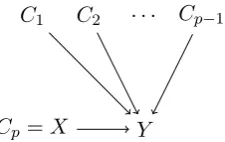
3.1 A graphical representation of the form of the models used in variable

selection in Chapter 3 for joint effects of multiple covariates. . . 60

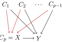
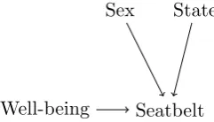
3.2 A graphical representation of the form of the models used in model

selection in Chapter 3 for joint confounding by multiple factors. . . . 62

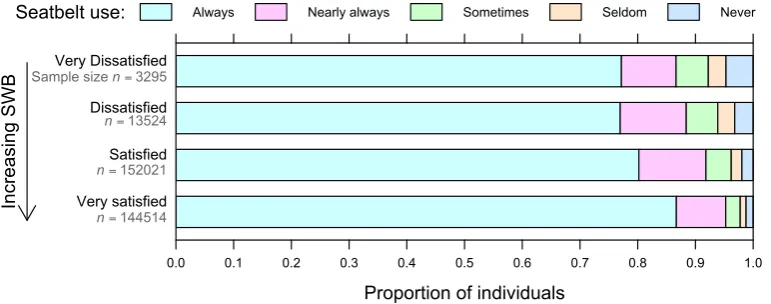
3.3 Frequency of seatbelt use cross-tabulated by subjective well-being

(SWB). . . 64

3.4 The model selected by variable selection for seatbelt use for joint

effects of multiple covariates. . . 66

3.5 Fitted (posterior) probabilities of always wearing a seatbelt given

subjective well-being. . . 67

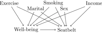
3.6 The model selected for joint confounding by multiple factors of the

relationship between well-being and seatbelt use. . . 68

4.1 Illustrative graphs of when small local moves may fail to enable

tran-sitions between two regions of high probability. . . 85

4.2 An illustrative example of the notation used in defining the two-stage

sampling for the Gibbs sampler. . . 94

5.1 ROC curves given by estimated posterior distributions from 10

repli-cations of our Gibbs sampler, MC3, and the REV sampler for the

(12)

5.2 The distribution of the areas under the ROC curves for the synthetic

data from the ALARM network, forn= 100, . . . ,5000. . . 114

5.3 Convergence diagnostics for all three MCMC samplers for the ALARM

data withn= 1000. . . 116

5.4 Convergence diagnostics for all 10 runs of each MCMC sampler for

the ALARM data withn= 1000. . . 117

5.5 Major discrepancies between pairs of the 10 independent runs for each

MCMC sampler. . . 118

5.6 Convergence diagnostics for all three MCMC samplers for the BRFSS

data. . . 121

5.7 Convergence diagnostics for all 10 runs of each MCMC sampler for

the BRFSS data. . . 122

5.8 Stability of estimators of the BRFSS data across bootstrapping, as

measured by SHDs, with the graph density made to match the graph

given by the PC-algorithm. . . 124

5.9 Convergence diagnostics for all three MCMC samplers, for the flow

cytometry data. . . 126

5.10 Stability of estimators for the flow cytometry data across

bootstrap-ping, as measured by SHDs, with the graph density made to match

the graph given by the PC-algorithm. . . 128

6.1 Convergence diagnostics for MC3 and the Gibbs sampler for the Add

Health data. . . 138

6.2 Summary network for the Add Health variables considered. . . 141

6.3 Conditional probability of depression, given various covariate states. 142

B.1 Log scores of the graphs visited by the three MCMC samplers in 10

(13)

B.2 Major discrepancies between pairs of the 10 independent runs, for

each MCMC sampler on the BRFSS data. . . 158

independent runs on the BRFSS data. . . 159

independent runs on the flow cytometry data. . . 160

B.5 Stability of estimators for the BRFSS data across bootstrapping, as

measured by SHDs, with the graph density made to match the graph

given by the Xie-Geng method, or so that the threshold is 0.5. . . . 161

B.6 The edges with posterior edge probability greater than 0.5, as given

by the Gibbs sampler for the BRFSS data. . . 162

B.7 Major discrepancies between pairs of the 10 independent runs, for

each MCMC sampler on the flow cytometry data. . . 162

B.8 Convergence diagnostics for all 10 runs of each MCMC sampler for

the flow cytometry data. . . 163

B.9 The edges with posterior edge probability greater than 0.5, as given

by the Gibbs sampler for the flow cytometry data. . . 164

B.10 Stability of estimators for the flow cytometry data across

bootstrap-ping, as measured by SHDs, with the graph density made to match

the graph given by the Xie-Geng method, or so that the threshold is

(14)

List of Notation

Basics

n The number of observations . . . 14

p The number of variables . . . 14

y A n-dimensional vector random vector . . . 13

Θ The parameter space of the entire model . . . 13

θ A vector parameterθ∈Θ . . . 13

X A n× p matrix of data, or the collection of random vectors {X1, . . . , Xp} . . . 20

XA The columns ofX specified by A . . . 34

X₋i The columns ofX except column i . . . 20

⊥⊥ Independence of random variables. . . 18

⊥⊥ Dependence of random variables. . . 18

O Complexity upper bound. . . 90

(15)

N Normal distribution . . . 25

MVN Multivariate normal distribution . . . 30

IG Inverse-gamma distribution . . . 25

Models M A finite set of models . . . 15

M A model from the set of modelM . . . 15

|M| The number of models . . . 15

pM The dimension of model M . . . 14

ΘM Parameter space under model M . . . 15

θM The parameters of model M . . . 15

p(y|θM) The likelihood of model M . . . 15

π(θM |M) Parameter priors under model M . . . 15

π(M) Prior weight for model M . . . 15

p(y|M) The marginal likelihood of model M . . . 16

p(M |y) The posterior model distribution . . . 15

MMAP _{The maximum}_{a posteriori} _model _{. . . .} ₁₆

Graphs G The set of all directed, acyclic graphs (DAGs) with p nodes 20 G= (V, E) A mathematical graph . . . 18

V Vertices . . . 18

(16)

Gij The (i, j) element of the adjacency matrix . . . 19

p The number of nodes in the graph G . . . 18

The number of edges in the graph G . . . 90

(i, j) Directed edge from node ito node j . . . 18

i→j Directed edge from node ito node j . . . 18

j←i Directed edge from node ito node j . . . 18

Gj The parents of node j inG . . . 18

hG1, . . . , Gpi The graphG with these parent sets. . . 19

GA The parent sets inG of nodes in A . . . 19

G₋A The parent sets inG of nodes not in A . . . 19

TG Transitive closure matrix for G . . . 90

CG A path count matrix for G . . . 91

ν(G) The set of neighbouring graphs of G . . . 48

G−_ij The graphG, with no edge i→j . . . 82

G+_ij The graphG, with an edge i→j . . . 82

d The number of nodes in a path . . . 19

Bayesian networks G A Bayesian network. . . 20

XGj The random variables corresponding to the parentsGj of nodej inG . . . 20

(17)

π(G) Prior for graph G . . . 39

πi(Gi) Prior for the parents of node iin graphG . . . 79

p(X|G) The marginal likelihood for G . . . 39

p(Xi|XGi) The local marginal likelihood . . . 80

κ The maximum in-degree . . . 41

Regression models γ Indicator variable for the included predictors. . . 27

Mγ Regression model, with predictors indicated byγ . . . 27

pγ The number of predictors in modelMγ . . . 27

Xγ Matrix formed from the columns of X corresponding to predic-tors inMγ. For normal linear regression, the matrix also includes a column of 1s. . . 27

Discrete data r The number of categories (or levels) of y . . . 24

nk The number of observations in the kth category . . . 25

C_jγ jth configuration under modelMγ . . . 27

qγ Cardinality of the sample space of Xγ . . . 27

Normal data m,mγ The prior mean (under model Mγ) . . . 25

v,Vγ The prior variance (under model Mγ) . . . 25

(18)

wj The jth node inW . . . 93

ρ The number of nodes in W . . . 86

F_W The collection of parent sets of W that yield an acyclic graph. . . 87

FW The collection of parent sets of nodes inW . . . 86

Fwj The parents in FW of the node wj inW . . . 86

F The set of acyclic graphs that differ from G in the parents of nodes inW . . . 93

P(FW |G−W,X) The conditional distribution for the parents of nodes in W . 87 H The set of all DAGs on the nodes in W . . . 93

H A DAG on the nodes in W . . . 93

η The number of nodes in H . . . 93

FHh A component of a partition of F. . . 93

G− The graph formed from Gby removing edges directed towards a node in W . . . 93

Dj The descendants of node wj ∈W inG− . . . 93

Kj The non-descendants of node wj ∈W inG− . . . 93

K Nodes that are not descendants in G− of any node inW . . 93

D_jH Descendants inG− of nodes in Hwj . . . 93

FH_W The collection of allowed parent sets for each nodewj ∈W, using H . . . 98

(19)

FH_j The set of allowed parent sets for wj, using H . . . 98

G_j The set of possible parent sets of node j . . . 99

Gi_j The G_j that contain node i . . . 99

⊗ Outer matrix product . . . 91

(20)

Acknowledgements

I am very grateful to my supervisors, Sach Mukherjee and Frances Griffiths, for

their constant enthusiasm, encouragement and inspiration throughout my time at

Warwick. It has also been a pleasure to collaborate with three economists (Andrew

Oswald, Jan-Emmanuel De Neve and Stephen Wu) and I am particularly grateful

for their efforts in helping a statistician to understand some of their field.

I have been fortunate to work amongst many other generous and friendly members of

staff and students at the Department of Statistics. Thank you particularly to those

in Sach’s group, those who suffered me in D0.06, and to Chris Jewell who ran the

departmental high performance computing facilities in his own time so pleasantly.

I am indebted to my parents and sisters for their encouragement and support. Most

importantly, I thank Sarah, my fianc´e and closest friend, who experienced the

devel-opment and writing of this thesis the most closely, but was nevertheless supportive

and encouraging throughout.

I also thank Marco Grzegorczyk, Dirk Husmeier, Karen Sachs, Amanda Goodall,

Graham Loomes, and Mark Steel for an assortment of thoughts, code and data

used in various parts of this thesis. Financially, I have been been supported by a

joint Economic and Social Research Council (ESRC) and Engineering and Physical

(21)

Declarations

I hereby declare that this thesis is based on my own research, except when stated

otherwise. This thesis has not been submitted for a degree at another university.

Some of this work has been published, is available as a working paper, or has been

submitted for publication as follows.

The material of Chapter 3 forms part of a paper ‘Happiness as a driver of

risk-avoiding behavior’ that is under review, co-authored with Sach Mukherjee,

Jan-Emmanuel De Neve, Andrew J. Oswald and Stephen Wu. The analyses from this

paper presented here are my own work, although an initial ordinary least squares

analysis was conducted by Stephen Wu. An earlier version of this paper is available

as CESifo Working Paper Series No. 3451.

Chapters 4 and 5 are an extension of work available as CRISM Working Paper

No. 11-21, under the title ‘An efficient Gibbs sampler for structural inference in

Bayesian networks’. The working paper is co-authored with Sach Mukherjee.

The material presented in Chapter 6 was published as ‘Exploratory network analysis

of large social science questionnaires’ in the Proceedings of Bayesian Modelling

Applications Workshop (BMAW-11). This was co-authored with Sach Mukherjee

(22)

Abstract

Structural inference for Bayesian networks is useful in situations where the under-lying relationship between the variables under study is not well understood. This is often the case in social science settings in which, whilst there are numerous theories about interdependence between factors, there is rarely a consensus view that would form a solid base upon which inference could be performed. However, there are now many social science datasets available with sample sizes large enough to allow a more exploratory structural approach, and this is the approach we investigate in this thesis.

In the first part of the thesis, we apply Bayesian model selection to address a key question in empirical economics: why do some people take unnecessary risks with their lives? We investigate this question in the setting of road safety, and demon-strate that less satisfied individuals wear seatbelts less frequently.

Bayesian model selection over restricted structures is a useful tool for exploratory analysis, but fuller structural inference is more appealing, especially when there is a considerable quantity of data available, but scant prior information. However, robust structural inference remains an open problem. Surprisingly, it is especially challenging for largenproblems, which are sometimes encountered in social science. In the second part of this thesis we develop a new approach that addresses this problem—a Gibbs sampler for structural inference, which we show gives robust results in many settings in which existing methods do not.

(23)

Chapter 1

Introduction

The aim of statistical modelling is to improve the degree of understanding of a

phenomenon of interest. Statistical models can help to describe and explain many

things including which factors are important; the direction and magnitude of the

associated effects; and, more generally, the relationship (if any) between variables of

interest. However, the level of precision that is attainable with statistical analysis

is usually determined by the nature of the data that are available and the (a priori)

assumptions one is prepared to make.

In general, more precise inferences will be possible when more data are available.

The sample size is usually the most important dimension of the data. In addition,

for the analysis to be useful, it will typically be important that the data are a

representative sample from the larger population under study, to facilitate inference

about the wider population. The second dimension of the data (the number of

variables measured) is also important because of the need to minimise the possibility

that a factor that was not measured performs an important role in the system under

study.

(24)

is the existing level of understanding. Statistical inference is always built upon

assumptions. In likelihood-based inference, many of the important assumptions are

made when determining the likelihood. In some settings, these assumptions may be

based upon accepted theories of the underlying system and are thus well founded.

In such a case, inference is about understanding the details of a system for which

the structure is already understood. In multivariate statistics, a core part of these

assumptions relate to the dependencies between different variables (or components)

of the system. Any assumption made about the structure of the dependency is

important in statistical inference because it is built into the likelihood.

1.1 Scope of the analysis

In this thesis, we consider the situation in which high-quality data are available,

but the existing accepted level of understanding of the phenomenon under study is

poor. In particular, we mostly do not assume a particular structure of dependence

between the components of the system. Instead, the purpose of the analysis is to

make inference about dependence. Making relatively weak assumptions, such as we

do here, means that we keep an open mind to unexpected relationships. Thus the

analysis that we make is mostly exploratory in nature.

We also assume that only observational data are available. In such cases, without

any information about the effect of interventions, it usually is very difficult to infer

anything conclusive about causality. There is a large literature covering methods

for analysing data collected through observational studies (Rosenbaum, 2002), but

much of this avoids making causal claims. Some of the strongest claims about

causality have come from researchers working with graphical models, for example,

Cox and Wermuth (2004), and, most prominently, Pearl (2009). However, it remains

(25)

there are many advocates of other approaches (notably Rubin, 2005).

Here, we take the view that graphical approaches are useful tools in situations in

which strong causal claims are sought, but we do not seek to construe our results in

this manner. Instead, we view our work as primarily about discovering relationships

that suggest interesting conjectures; these are framed in a manner that allows further

work (ideally interventional) to be carried out to examine the conjectures in more

detail. This point of view has been proposed previously by many authors including

Williamson (2005), who views the approach as a hybrid between a

hypothetico-deductive and an inductive approach to discovering causal relationships.

The cost of data collection is generally falling, and so ‘large’ datasets are now

in-creasingly the norm. A considerable amount of data are now available that describe

phenomena about which no consensus model is available. Datasets describing

var-ious aspects of economics, genetics, molecular and cell biology, and diverse areas

of the social sciences are widely available. In many of these areas, the growth in

the availability of data has exceeded the growth in theoretical understanding. This

opportunity is an opening for statistical methods that improve understanding in

these settings.

1.2 Statistical model selection

1.2.1 Inadequacy of the complete model

In poorly understood settings there may be many factors that could plausibly play an

important role in the system under study. In this situation a model that incorporates

all of these factors may seem attractive, because it incorporates all of the available

information and the analysis is not prejudiced by the disregarding of potentially

(26)

The estimator associated with thiscomplete orfull modelwill have many

de-grees of freedom, and so it is able to closely replicate features in the data. However,

the ‘volume’ of space in which a high-dimensional probability distribution may have

support (regions of positive probability) increases exponentially as its dimension

in-creases, a phenomenon described as the ‘curse of dimensionality’ by Bellman (1961)

in the context of dynamic programming. This effect results in the available data

being sparsely dispersed across the space relative to its size.

Another example of this problem is given by Silverman (1986), who calculates

the required sample size for an estimator ˆp(x) of the density p(x) at the origin

of a unit multivariate normal distribution to have relative mean squared error

E (ˆp(0)−p(0))2

/p(0)2 less than 0.1. For a univariate distribution p(x), only 4

samples are required to satisfy this criterion; for a 5-dimensional distribution, 768

samples are required; and for a 10-dimensional distribution, around 842,000 samples

are required. Thus even for a smooth unimodal distribution, with a simple

mea-sure of fit based around the mode of the distribution, the amount of data required

rapidly becomes enormous as the dimension of the distribution grows. As a result,

even with a large sample size, a single dataset in a high-dimensional setting will not

exhibit all of the characteristics of the underlying probability distribution.

Thus, while on average closely matching the data will give accurate estimates, rigidly

replicating the exact properties of a single dataset may be far from optimal. An

estimator that does this will be particularly susceptible to small variations in the

data, and so the estimator will have high variance. On the other hand, the estimator

has low bias because averaging across replications of the data will give accurate

estimates. Particularly in exploratory settings, the complexity of a model including

all of the factors is a disadvantage. For these reasons, the complete model is often

(27)

complete model whilst mitigating its disadvantages. The advantage that we want to

keep is the small bias; the disadvantage we seek to ameliorate is its large variance.

In these settings reducing variance will increase the bias, and so a trade-off exists

between these properties (see, e.g. Hastie et al., 2009). At the opposite end of the

spectrum of model complexity to the full model, we could consider a univariate

model that includes no covariates. This model will typically have the opposite

problem: large bias, but low variance.

A particular example of these trade-offs is a regression model with 100 potential

predictors. The ordinary least squares estimators for the regression coefficients are

consistent, so as the sample size grows, the coefficients will converge to their true

values. In practice, we have only a finite sample, and so the estimators will not give

the true values of the coefficients. In particular, the estimates for the coefficients

in the full model will have a large variance. The large variance in the estimates is

intuitive because in the parameter space for the full model, the data will be sparsely

dispersed, and so a small change to an individual data point may lead to a large

change in the estimators. Averaging across replications of the data, however, will

lead to the estimators having the correct values. Thus, the bias of the estimators is

low. In contrast, a model including only one predictor will have low variance, which

is intuitive because a relatively large amount of data will be used to estimate its

value. However, such a simple model may not be expressive enough to capture the

true form of the data, and so the bias of the estimator will be high.

1.2.2 Objectives and viewpoints

We have described why in many settings a full model may not be appropriate even if

it does subsume the ‘true model’ (the concept of a ‘true model’ is discussed further

below, in Sections 1.3.2 and 1.2.3). Conversely a simple, univariate model may not

(28)

an intermediate model that balances the competing requirements of minimising

bias and variance. The models that are considered may be of differing dimension or

contain different functional forms. Handling the varying dimensions of the models

considered is particularly difficult. The problem of finding an appropriate model is

known in general asmodel selection.

The ideal model will strike a balance of being consistent with the data without being

overly complicated in such a way that over-fitting will occur. This idea has a long

history and is often attributed to William of Ockham, under the name Occam’s

razor, or called theprinciple of parsimony. Each model may be associated with

a particular scientific hypothesis, and so model selection may be useful in comparing

the competing hypotheses.

One aim of model selection is to understand the dependence structure of the

vari-ables. The structure of the dependence within a system can be encapsulated by the

likelihood function of a statistical model. Inference about the dependence

struc-ture can thus be considered as statistical model selection. The origins of this form

of analysis can be traced back to the work of Sewall Wright, who developed the

method of path analysis (Wright, 1921), which aims to measure the direct effect

of each ‘path’ in a system. Another early methodology that can be viewed in this

light is that of Dempster (1972), in which the covariance structure of a multivariate

normal distribution is modelled with a particular focus on finding a simple

descrip-tion of its structure. A simple descripdescrip-tion of the structure is achieved by setting

appropriate entries of the inverse covariance matrix to zero. In doing so, conditional

independence, given all other variables, is implied between the corresponding

vari-ables, and the number of parameters in the model is reduced. These models can

be viewed as undirected Gaussian graphical models (Lauritzen, 1996). The models

considered in this thesis can be viewed as originating in similar work. However,

(29)

Bayesian networks.

1.2.3 What is a statistical model?

Before turning to practical issues related to choosing the model, we discuss the

meaning and role of statistical models and their relationship to ‘truth’. Bernardo

and Smith (1994, ch. 4, pp. 237) argue that most statisticians agree that the role of

models is to provide a focused framework within which simplified representations of

phenomena can be discussed. The most optimistic view is that a single statistical

model can encapsulate ‘truth’. Thus, if we can construct a list M of candidate models, we can try to determine which of these is true. This view usually seems

overly-optimistic. Instead, a more appropriate view in most contexts is the

prag-matic view taken by Box and Draper (1987) in a discussion of the bias-variance

trade-off: “all models are false, but some are useful”. Buckland et al. (1997) take

a similar view asserting that the ‘truth’ is high dimensional, and effectively infinite

dimensional, and so in handling model uncertainty we should seek the best

approx-imating fit rather than the ‘truth’. Another pragmatic viewpoint is taken by Fisher

and Neymann (as discussed by Lehmann, 1990), who suggest that the key

char-acteristic of models should be familiarity and simplicity. See Cox (1990) for more

discussion on the role of models.

1.2.4 Implementation of model selection

In practice, choosing a model that balances bias and variance is not straightforward.

For complex multivariate models, assessing the bias and variance associated with

an estimator from a single, finite dataset is challenging. In particular, measuring

the discrepancy between the observed data and a model is not sufficient because by

this metric the full model is always selected. In addition, the traditional methods of

(30)

maximum likelihood estimators (MLEs) do not give sensible results in this context

for several reasons.

One problem is multiple testing. Freedman (1983) examined this issue empirically.

Data from 50 independent random variables were regressed against data from an

entirely independent variable. Alarmingly, after dropping 35 variables which were

insignificant at 0.25 level, 6 of the remaining 15 variables were judged significant

at the 0.05 level. The Bonferroni correction (Bonferroni, 1936; Bland and Altman,

1995) offers a simple adjustment for this problem under an assumption of

indepen-dent tests. There has been much work on multiple testing in recent years (see e.g.

Benjamini and Hochberg, 1995; Dudoit and van der Laan, 2008).

Additionally, the metric by which we judge a model must account for the number

of parameters that the model includes. One approach in the frequentist framework

is to add a term to the likelihood function that penalises high-dimensional models.

Examples include Akaike’s information criteria (Akaike, 1974; Burnham and

Ander-son, 2002), which is known as AIC, and the Bayesian information criteria (Schwarz,

1978), which is known as BIC. Information criteria describe a general method for

likelihood penalisation. Penalised likelihood approaches for model selection have a

rich literature, see e.g. Claeskens and Hjort (2008). We describe AIC and BIC in

more detail in Section 2.1.

In the specific context of regression, penalisation based on `1 and `2 norms of the

coefficient vector are widely used (B¨uhlmann and van de Geer, 2011). Ridge

re-gression (Hoerl and Kennard, 1970) uses a `2 penalty. Using this penalty allows

straightforward maximisation of the (penalised) likelihood to yield a closed-form

estimator. The estimates for the regression coefficients are shrunk towards zero,

thereby controlling over-fitting. However, ridge regression does not set regression

(31)

se-estimates for the regression coefficients to exactly zero. Here, maximisation of the

penalised likelihood requires optimisation, but an efficient algorithm called LARS

(Efronet al., 2004) exists.

Bayesian model selection offers an alternative approach (detailed in the next

sec-tion). Rather than directly using penalised likelihoods, a posterior distribution

across a set of models is constructed, and comparison between pairs of models can

be made using Bayes factors. Bayesian model selection and penalised likelihood

methods are closely related: the log posterior distribution is given, up to a

con-stant, by the sum of the log likelihood and the log prior. The (negative) log prior

can therefore be viewed as a penalty term. This view makes clear the relationship

between various penalised likelihood estimators and related Bayesian formulations.

Approaches that draw ideas from the Bayesian approach in a frequentist context are

also available. For example, Buckland et al. (1997) propose a method for

assign-ing weights to models, but the weights arise from functions of information criteria,

rather than from a posterior distribution. The BIC also straddles both frameworks:

although it takes the form of a penalised likelihood, it is also an asymptotic

approx-imation to the Bayes factor.

1.3 Bayesian model selection

1.3.1 Basic Bayesian framing

Model selection in the Bayesian framework considers an indicator variable over

mod-els as an additional parameter, equipped with a prior and posterior distribution in

the same way that all parameters do in the Bayesian framework. The usual

(32)

models can then be found by an application of the discrete version of Bayes’

the-orem. The theory of handling model uncertainty in a Bayesian framework is now

well-developed; Clyde and George (2004) give a full overview.

1.3.2 Interpretations of Bayesian model selection

The interpretation of Bayesian model selection is clearest when one of the models

is viewed as the ‘truth’. Usually this seems unrealistic, but in practice, especially

when|M|is large, this may be a sufficiently good approximation. Assuming one of the models inMis true is calledM-closed by Bernardo and Smith (1994), who also delineate two further perspectives that could be taken on the list Mof models. In theM-completed viewpoint none of the models inMis viewed as true because our true beliefs can only be represented by a separate modelMt, which is precluded from

direct consideration by intractability. In this setting we need to proceed differently

because it does not make sense to assign a prior toMwhen this would not represent our true prior beliefs. The final possibility, M-open, occurs when even specifying

M_t is not possible. For the settings considered here, an M-open viewpoint is the most plausible, but for pragmatic reasons we will generally work in a relatively

M-closed framework.

1.3.3 Practical implementation

In the previous section, we noted the difficulty in comparing models of different

dimension, because unadjusted measures of fit will invariably prefer the most

com-plex model. In the Bayesian formulation, the relative posterior weights assigned to

two models is determined by the Bayes factor, which is the relative marginal

likeli-hood. Comparison of models of differing dimension is possible because the marginal

(33)

The computation of the posterior model distribution is often challenging, and

ad-dressing this in a particular context forms a key part of this thesis. Simpler

alter-natives have been proposed. For example, Draper (1995) considers starting from a

single model, and expanding it as suggested by context or the data. However, in the

context we consider here, it is attractive to consider a fully-Bayesian approach

be-cause the high-dimensionality makes it difficult to propose a sensible starting model.

Another simplification that can be often useful is BIC, which is an asymptotic

ap-proximation to the posterior distribution.

1.3.4 Summarising the posterior distribution

Once the posterior distribution over models has been evaluated, two distinct

ap-proaches can be taken to summarising its contents.

A simple approach is to find the posterior mode. The modal model (or models) is

the model that is most consistent with the data. While simple and convenient, a

drawback to this approach is that a level of uncertainty is ignored because it implies

that the final results are made conditional on the modal model (e.g. Chatfield, 1995).

When a quantity of interest that is interpretable across all the models under

con-sideration can be extracted from each model an alternative approach is available.

In this case, it follows from Bayes’ theorem that the posterior distribution for this

quantity is given by taking its average across the models, weighted by the posterior

mass for each model.

1.3.5 Bayesian model uncertainty in social science

Bayesian approaches to model uncertainty have not been widely adopted in social

science, despite the significant model uncertainty that exists. The foremost

(34)

research is Raftery (1995). In econometrics, Fern´andez et al. (2001b) advocated

Bayesian model averaging as a principled way to account for model uncertainty in

cross-country growth regression.

1.4 Contributions of the thesis

The thesis consists of three main contributions.

The first contribution is a study of the effects of well-being on risk-taking. This

question has not been considered before, although Kirkcaldy and Furnham (2000)

found correlations consistent with the findings of our work. We take a Bayesian

model selection approach to the question, which is unusual in empirical economics.

We find evidence in support of the theory that those with higher levels of well-being

are more averse to risk-taking.

We then introduce a novel Gibbs sampler for structural inference of Bayesian

net-works. While Gibbs samplers have been used with Bayesian networks before, they

have not been used for structural inference. The Gibbs sampler introduced here

explores the posterior distribution of Bayesian networks. While the general method

of Gibbs sampling is well-established, the requirement of acyclicity in Bayesian

net-works makes designing a Gibbs sampler difficult in this context. We show

empiri-cally that the Gibbs sampler exhibits far superior performance compared to several

state-of-the-art methods. Indeed, in many cases, results obtained from widely used

methods are so unstable as to be unusable in practice.

The final contribution of the thesis is an explorative study of depression in

adoles-cents. Large social science questionnaires, including the survey we use in the thesis,

have not been previously studied using structural inference of Bayesian networks.

(35)

Chapter 2

Background

2.1 Model selection

A parametric statistical model does not fully describe a probability distribution.

Instead, it describes a family of distributions, up to some parameters θ. For a

vector valued random variabley, a modelM specifies the joint distribution ofy, up

to unknown parameters θ. The joint probability of y can be specified conditional

on both parametersθand model M.

p(y|θ, M) withθ∈Θ

Often, dependence on the modelM is left implicit and emphasis placed on the joint

distribution as a function of parameters θ, i.e. the likelihood function.

Statisti-cal inference seeks to understand the relationship between these parameters, and

data. In Bayesian inference, we aim to describe the posterior distribution of these

parameters, given the data.

(36)

As outlined in Chapter 1, we will be considering a situation in which observations

of many variables are available, but the appropriate model for the variables is not

known. Therefore, we will consider the model itself as the object of interest for

inference.

Supposensamples frompvariables are available. LetpM be the dimension of model

M.

In the frequentist framework, a widely used approach to model selection involves

pe-nalised likelihood methods. The most well-known of these, the AIC, was introduced

by Akaike (1974) and has the following form.

−2 log(p(y|θ, M)) + 2pM

The model that minimises AIC is preferred. An alternative is the Bayesian

Infor-mation Criterion (BIC), introduced by Schwarz (1978).

−2 log(p(y|θ, M)) +pMlog(n)

In the specific context of regression, numerous penalised estimators for the regression

coefficients β have been proposed. Consider a regression model for an outcome

variabley, using a set ofqpredictors. Suppose we have observationsy= (y1, . . . , yn)

of the outcome, and observations of the predictors arranged into the columns of

a matrix X. The LASSO (Tibshirani, 1996) penalises the regression coefficients

by an `1 penalty. This penalty permits setting of some regression coefficients to

exactly zero, thereby leading to variable selection. An older alternative is ridge

regression (Hoerl and Kennard, 1970), which uses an `2 penalty, and yields the

following estimators for the regression coefficients, with Iq being the q×q identity

matrix.

ˆ

(37)

While ridge regression will shrink coefficients towards zero, it will not shrink them

to exactly zero in the way the LASSO does, and so does not lead to variable

selec-tion directly. Numerous other penalties have been proposed, notably the smoothly

clipped absolute deviation (Fan and Li, 2001), the elastic net (Zou and Hastie, 2005)

and the adaptive LASSO (Zou, 2006).

The Bayesian approach does not use a penalised likelihood explicitly, but the log

prior can be viewed as such. A particular instance in which the two approaches yield

the same solution is a regression in which the prior for the regression coefficients

is β ∼N(0, σ2λ−1Iq). The resultingmaximum a posteriori (MAP) estimator forβ

matches the ridge estimators exactly (Hoerl and Kennard, 1970; Hsiang, 1975).

2.1.1 Bayesian model selection

The Bayesian approach to model selection treats the model simply as another

pa-rameter. Suppose a finite set of modelsMis under consideration, and that a vector of observationsy is available. Each modelM ∈ Mconsists of a likelihood function p(y|M, θM) with parameters θM ∈ΘM. These parameters have priorsπ(θM |M)

in each model.

Since the set of modelsM under consideration is a finite set, the model prior is a discrete distribution over this set.

π(M) =πM, M ∈ M where πM ≥0 and X

M∈M

πM = 1

An expression for the posterior distribution for a model M can be written down

immediately, by a simple application of Bayes Theorem. The expression depends

on the marginal likelihoodp(y|M) of M.

P(M |y) = P p(y|M)π(M) M∈Mp(y|M)π(M)

(38)

The quantityp(y|M) is given by

p(y|M) = Z

ΘM

p(y|M, θM)π(θM |M)dθM, (2.2)

and is referred to as themarginal likelihood.

Evaluation of this posterior distribution is typically difficult for two reasons. First,

the integration in Equation 2.2 may be difficult to evaluate. This difficulty motivates

the use of conjugate models, as described in Section 2.3.1, which enable evaluation

of the integral analytically. The second difficulty is the summation over M in the normalising constant of Equation 2.1. When the cardinality of M is large, it is not possible to evaluate the summation exactly. However, Markov chain Monte

Carlo methods enable the posterior distribution to be approximated without directly

evaluating the normalising constant.

There are two distinct approaches for summarising the posterior distribution. A

simple approach is to select a single model, and base any further inference as

condi-tional upon this model. When choosing a single model, the maximuma posteriori

(MAP) model is usually chosen.

MMAP_{= arg max}

M P(M |y)

The MAP modelMMAP _{may not be unique, and even when it is, it may not be}

rep-resentative of the posterior distribution. If the posterior distribution is multi-modal,

with disparate models having high posterior probability, it may be unsatisfactory

to choose the one model.

Alternatively, if some quantity ∆ is interpretable in all models, we can average it

across all of the models, weighting by the posterior model probability.

(39)

This approach is called Bayesian Model Averaging (Hoetinget al., 1999; Wasserman,

2000). Choosing an appropriate model prior can be challenging, and is discussed

further in Sections 2.4.3 and 2.5.4.

2.2 Graphical models

Throughout this thesis, the relationship between variables is studied using graphical

models. These models enable the decomposition of complex multivariate

distribu-tions into simpler local distribudistribu-tions. Such a decomposition can reveal a great

deal about the relationships between the variables. In addition, a graphical model

provides a statistical and computationally tractable description of a large joint

dis-tribution.

The decomposition is formed by the conditional independence structure, which can

be represented by a graph. Thus, graphical models describe families of probability

distributions using a mathematical graph. The graphical representation can ease

the interpretation and clarify the structure of complex models. In addition, in some

situations, the computation of particular marginal distributions can be simplified

when a graphical representation is considered (see e.g. Lauritzen and Spiegelhalter,

1988).

In most graphical models, the nodes of the graph represent random variables and

the edges represent the (conditional) dependence structure amongst the random

variables. The conditional independence structure gives a deeper understanding of

the relationships between the random variables, as we describe below.

A variety of graphical models have been developed (see e.g. Lauritzen, 1996; Smith,

2010). The two most widely used graphical models are Markov random field models,

which are represented by an undirected graph, and Bayesian networks, which are

(40)

model.

2.2.1 Conditional independence

While a crude understanding of the relationship between random variables is

pro-vided by a simple correlation analysis, a far deeper understanding is propro-vided by

the conditional independence structure. In particular, correlation analysis gives no

understanding of whether relationships between two variables are mediated by a

third, whereas this is captured in the conditional independence structure. Such

knowledge is generally informative, and indeed much of statistics can be considered

in terms of conditional independence (Dawid, 1979). Knowledge of the conditional

independence structure is particularly valuable when a loose form of causality is

sought.

Two random variablesAandB are conditionally independent given a third random

variableC if the following property holds.

p(A, B|C) =p(A|C)p(B|C) for all C such thatp(C)>0

When this property holds, we use the shorthandA ⊥⊥B |C. We write A ⊥⊥B |C

when the property does not hold.

2.2.2 Graphs

A mathematicalgraphG= (V, E) consists of a set ofnodesV = (1, . . . , p), and a

set ofedgesE that link pairs of nodes. We also usev1, . . . , vp to denote the nodes

in the graph.

(41)

and will use three different notations to specify their edges: the collection of edges;

adjacency matrices; and parent sets.

First, we can specify edges of a graph as a subsetE ⊆V ×V, as per the definition of a graph. Individual directed edges from node i to node j can thus be denoted

by either the pair (i, j), or the symbol i→j. We will refer toi as thehead of the edge, andj as the tail.

We can also specify the graphG= (V, E) with anadjacency matrix G, ap×p matrix with elementsGij given by

Gij = 

 

 

1 if (i, j)∈E 0 otherwise.

The final specification of the edge set E of the graph Gthat we use is in terms of

the parents Gj of each node j, forj ∈ {1, . . . , p}. The parents Gj of node j are

the subset of nodesV such that i∈Gj ⇔(i, j) ∈E. We refer to Gj as a parent set.

It will sometimes be convenient to use the collection of parent setshG1, . . . , Gpi to

specify a graphG. Subsets thereof are denoted by GA=hGk : k∈Ai. ThusGA is

a collection of parent sets, specifying only the parent sets of nodes inA; the parent

sets of nodes not inAare not specified byGA. The subset given by the complement

AC = {1, . . . , p} \A of a set A is denoted by G₋A = hGk : k ∈ ACi. Thus G−A

specifies the parent sets of nodes not in A, leaving the parent sets of nodes in A

unspecified. The parent sets of all nodes can be specified byhGA, G−Ai. Thus, in

particular, any graph G can be specified as hGj, G−ji = hG1, . . . Gpi = G for any j∈ {1, . . . , p}.

(42)

for each i = 1, . . . , d. In a directed graph, we usually require that (vi−1, vi) ∈ E

meaning that the path obeys the directions of the edges. However, it will occasionally

be useful to consider a path that does not obey the direction of the edges on a path.

Cycles are a particular type of path that will be of key interest. A cycle is path

v0, v1, . . . , vd, d ∈ N, such that v0 = vd, and the path obeys the direction of the

edges. A graphG in which a cycle exists is called cyclic; a graph without cycles

is called acyclic. We denote the set of all directed, acyclic graphs (DAGs) withp

nodes byG.

For undirected graphs, we denote byi−j an edge between node iand nodej. We define adj(i) as the set of nodesjsuch thati−j. Acomplete undirected graph is an undirected graph in which an edge links every pair of nodes in the graph.

2.2.3 Bayesian networks

Bayesian networks are a particular type of graphical model. A Bayesian networkG

is a DAG with nodes V = (1, . . . , p), and directed edges E ⊂ V ×V. The nodes correspond to the components of the random variables X1, . . . , Xp. We denote by

XGj the set of random variables that correspond to the parentsGj of nodej in the

graphG. It is convenient to refer to XGj as theparents of Xj.

A defining feature of Bayesian networks is that the joint distribution of X is

spec-ified in terms of p(Xi | XGi, θi), the conditional distribution of each Xi, given

its parentsXGi in the Bayesian network, with parameters θi. Denoting by X−i =

{X1, . . . , Xi−1, Xi+1, . . . , Xp}the random vector excludingXi, we havelocal mod-els(orlocal distributions) p(Xi|XGi, θi) that satisfy the following.

(43)

product of these local distributions.

p(X1, . . . , Xp |G) = p Y

i=1

p(Xi|XGi, θi)

The conditional dependence structure of the probability distribution can be

deter-mined using the d-separation criterion (Verma and Pearl, 1990). We describe this

criterion using the concept of blocked paths, which uses the concept of a path being

head-to-head at a node. We say that a path v0, . . . , vd (not necessarily obeying

edge directions) on a DAG G = (V, E) is head-to-head at a node vi, for some

i∈ {1, . . . , d−1}if (vi−1, vi)∈E and (vi+1, vi)∈E.

A blocked path can then be defined as follows. LetS be a subset of V so thatS is

a set of nodes in the graph. A path (not necessarily obeying edge directions) from

node v0 ∈ V to nodevd ∈V in a DAGG is said to be blockedby S if the path includes a nodevi, i∈ {1, . . . , d−1}, such that one of the following two criteria is

satisfied.

• vi ∈S and the path from nodev0 to nodevd is not head-to-head at nodevi. • The path is head-to-head at nodevi, and neither is node vi in S, nor does S

contain any of the descendants in the graphG of nodevi.

Two subsetsA, B⊆V ared-separated if all the paths (not necessarily obeying edge directions) fromA toB are blocked.

A particular conditional independence structure can be implied by multiple different

Bayesian networks. However, we can define an equivalence class on the space of

Bayesian networks such that Bayesian networks within the same class imply the

same conditional independence structure. The definition arises from the definition

ofd-separation and uses the concept of the skeleton of a Bayesian network, and ofv

-structures. Theskeletonof a Bayesian network is the undirected graph formed by

(44)

is defined as an ordered triple (i, j, k) of nodes, such thati→j and k→j, but no edge exists linking nodesiand kdirectly. Two Bayesian networks areequivalent

if they share the same skeleton andv-structures (Verma and Pearl, 1990).

We can specify the equivalence class of a Bayesian network using a completed

partially-directed acyclic graph (CPDAG). This name originates in Chickering (2002),

but the idea has been used by other authors under a variety of names. A CPDAG is

a partially-directed graph, whose directed edges do not form a cycle. For a Bayesian

networkG, CPDAG(G) is formed by considering all of the edgesE0 for which in all

graphs G0, such thatG and G0 are equivalent, that edge is oriented as in G. Then

CPDAG(G) is formed by removing the direction attached to each edge not in E0.

Chickering (2002) show that CPDAGs uniquely represent an equivalence class of

Bayesian networks.

2.3 Univariate Bayesian models

The basic building-blocks of the models that we consider in Section 2.4 and 2.5 are

simple univariate models. In this section, we first describe conjugacy, a property that

characterises a class of analytically-tractable models. We then review the simplest

form of the two conjugate models that are considered throughout this thesis.

We assume that Y is an n-dimensional random vector consisting of independent,

identically distributed components. We suppose observationsy ofY are available.

2.3.1 Conjugate priors

The integration required to evaluate Equation 2.2 is analytically intractable for

many choices of priors for a given model. If our understanding is such that our prior

(45)

a prior for which the integration is straightforward, this difficulty can be avoided.

For the models that we consider in this thesis, priors of the required form are well

known, and are calledconjugate priors.

Conjugate priors (Raiffa and Schlaifer, 1961) are familiesP of distributions that are closed under sampling from a distribution in a familyF of distributions. A familyP

of prior distributions is said to be closed under sampling from a distributionp(y|θ) in a parametric family F if for every prior distribution π(θ) ∈ P, the posterior distribution p(θ | y) ∝ π(θ)p(y | θ) is also in P. A catalogue of many conjugate priors is given in Gelmanet al. (2004).

Raiffa and Schlaifer (1961) list three properties that they view as desirable in a

family of priors: tractability, interpretability and richness. Conjugate families are

tractable, and this is the main reason for their adoption. Conjugate priors sometimes

also have a simple interpretation. In exponential families we can consider the prior

as constituting “virtual samples” (see, e.g. Robert, 2007), and so the relative weight

implied on the prior and data can be ascertained. It is in richness, however, that

conjugate families can be lacking. Ideally, a prior should exactly match a Bayesian

modeller’s prior beliefs, but conjugate priors are often not flexible enough to allow

this to be fully achieved. Sometimes, a close approximation to prior beliefs can be

constructed within the conjugate family, but often a poor approximation is accepted

because of the computational advantages of conjugate priors.

In many standard Bayesian models, using non-conjugate priors is now feasible since

the emergence of easily available computationally-intensive approximations.

How-ever, in the setting considered here, non-conjugate priors are not viable for the

following reasons.

First, there are formidable computational challenges even when conjugate priors are

used. These challenges are considerably compounded by the use of non-conjugate

(46)

size of the data is large. The large sample size means that the prior will exert only

a minimal effect on the posterior distribution, thus making its exact specification

less important.

For these reasons, we use conjugate priors throughout.

2.3.2 Multinomial-Dirichlet

The standard Bayesian model for univariate multinomial data (e.g. O’Hagan and

Forster, 2004) will form the basis of the models we consider in this thesis. Consider a

random vectorY, each component of which takes one ofr discrete categories.

Sup-pose thatY is distributed according to a multinomial distribution, with parameter

vectorθ= (θ1, . . . , θr), withθ >0 and θ1+· · ·+θr = 1.

Y∼Mult(θ1, . . . , θr)

The conjugate prior for the vectorθis Dirichlet, with hyperparametersα= (α1, . . . , αr)

whereαk >0,k= 1, . . . r.

θ1, . . . , θr ∼Dir(α1, . . . , αr) withθ1, . . . , θr ≥0 and r X

k=1

θk= 1

The normalising factor in the Dirichlet likelihood is a ratio of gamma functions

Γ(α) =R∞

0 xα−1e−xdx, for which, in particular, Γ(α) = (α−1)! forα∈N.

p(θ1, . . . , θr) =

Γ(α1+· · ·+αr)

Γ(α1). . .Γ(αr) r Y

k=1

θαk−1 k

The mean isαk(Prk=1αk)−1 for each θk.

The posterior distribution of θ is parameterised in terms of a contingency table

(47)

thekth category,k= 1, . . . , r.

θ1, . . . , θr |y∼Dir(α1+n1, . . . , αr+nr)

The formulation simplifies in the natural manner for binomial data with beta priors.

In using this formulation, we are assuming that the data are independent,

identically-distributed draws from a multinomial distribution. It will often be the case that some

heterogeneity exists and so it is more appropriate to use a model that is conditional

on some collection of covariates; we consider this possibility in Section 2.4.1.

2.3.3 Normal inverse-gamma

The models for normally-distributed data that we consider will similarly build upon

standard univariate models (e.g. Gelman et al., 2004). Suppose we have a

ran-dom vectorY, components of which are independent random variables distributed

according to a normal distribution, with meanµand varianceσ2.

Y ∼N(µ, σ2)

When both µ and σ2 are unknown, the conjugate priors for µ and σ2 are normal

and inverse-gamma respectively.

µ|σ2 ∼N(m, v−1σ2) σ2 ∼IG(a, b)

The hyperparameters a and b are respectively the shape and scale parameters of

the inverse-gamma distribution. The hyperparametersm can be interpreted as the

(48)

distribution has density

π(σ2) = b

a

Γ(a)(σ

2₎−(a+1)_exp(₋_b/σ2₎_.

The joint prior for (µ, σ2) is thus normal inverse-gamma NIG(m, v, a, b).

π(µ, σ2) =

√

v

σ√2π ba Γ(a)(σ

2₎−(a+1)_exp

−2b+v(µ−m) 2

2σ2

By conjugacy, the joint posterior distribution for (µ, σ2) is also normal

inverse-gamma.

µ, σ2|y∼NIG(m?, v?, a?, b?) where, with ¯y= _n1Pn

i=1yi and s2=

Pn

i=1(yi−y¯)2, the parameters are

m?= mv+ny¯

n+v

v?= 1

n+v

a?=a+n

2

b?=b+1 2

s2+nv(¯x−m)

2

n+v

.

2.4 Model selection for Bayesian regression models

Regression models aim to characterise the relationship between a response variable

and a collection of predictor variables. The model for the response is specified

condi-tionally on the predictor variables. We consider situations in which the parametric

form of the conditional distribution is known, up to the choice of predictor

vari-ables. Model uncertainty in this context is therefore uncertainty about which set of

predictor variables should be used. The problem is known asvariable selection.

(49)

‘out-come’ values, and an×p random matrixx of observations ofp predictor variables. These observations come from a random vector Y, and a n×p random matrix X, the columns of which are random vectorsX1, . . . , Xp, respectively.

We aim to determine which subset of the predictors {X1, . . . , Xp}is best suited to

predictingY, the outcome variable. There are 2p subsets of the p predictors, each

of which corresponds to a possible model forY. A regression modelMγ is specified

using ap-dimensional indicator vectorγ = (γ1, . . . , γp), the ith component of which

takes the value 1 when theith variable is included in the model, fori= 1, . . . p. Let

Xγ = {Xi: γi = 1} be the set of predictor variables included in model Mγ, and pγ = Ppi=1γi be the number of predictors included in the model. We use Mγ to

refer to the set of all models. Note that the predictor variables are assumed to be

observed without error.

2.4.1 Multinomial-Dirichlet

Suppose each component of the response vectorYhasrlevels, or categories. We will

be considering models for the responseYspecified to be conditional on a subsetXγ

of the set of discrete variables{X1, . . . , Xp}. Each component ofXi, fori= 1, . . . , p,

has ri levels. We define the configurations of Xγ to be the components of its

sample space, for whichqγ=Qpi=1r

γi

i is the cardinality. We label the configurations

C_jγ forj= 1, . . . , qγ. We assume that observationsyand xfor the outcome random

vectorYand the predictor random variablesXrespectively are available; we denote

byxγ the observations for the predictors included in modelMγ.

For a particular modelMγ, we assume that the distribution of Y is independently

parameterised for different configurations ofXγ, the predictors in the model. Thus

(50)

smaller parameter spaces Θγ,j corresponding to the configurations of the predictors.

Θγ =

×

j=1,...,qγ

Θγ,j

Thus the likelihood factorises across configurations.

p(Y|Xγ, θγ,j, Mγ) = qγ Y

j=1

p(Y|Xγ =C_jγ, θγ,j, Mγ) with θγ,j ∈Θγ,j

This independence assumption means that no information is ‘shared’ about the

dis-tribution ofY between cases in which the configuration of the predictors differ, and

the model may be entirely different for different configurations. In particular,

lin-earity in the predictors is not a requirement for the fitted model. This unstructured

form of model means that availability of a large sample size is important for useful

inference to be possible.

The distribution ofY conditional on the configurationC_jγ of the predictors is

spec-ified to be multinomial for each configuration, with j = 1, . . . , qγ, and with an

r-dimensional parameter vectorθγ,j ∈Θγ, each component of which corresponds to

a category ofY.

Y|Xγ, θγ,j, Mγ ∼Mult(θγ,j,1, . . . , θγ,j,r) forj= 1, . . . , qγ

The likelihood for y under a modelMγ is a function of the random variableNγ,j,k

given by the number of times that the predictors take thejth configurationC_jγ and

the outcome variable has thekth category, forj = 1, . . . , qγ and k= 1, . . . , r.

p(y|Xγ, θγ, Mγ) = qγ Y

j=1

r Y

k=1

θ_γ,j,kNγ,j,k

(51)

1, . . . , qγ.

θγ,j,1, . . . , θγ,j,r ∼Dir(αγ,j,1, . . . , αγ,j,r) withθγ,j,1, . . . , θγ,j,r ≥0, r X

k=1

θγ,j,k= 1

We assume thatθγ,j are a priori independent. This assumption, when taken with

the assumption that the distribution ofy is independently parameterised, is called

local independence (Spiegelhalter and Lauritzen, 1990). The joint prior for

(θγ,1, . . . , θγ,qγ) is thus the product of Dir(αγ,j,1, . . . , αγ,j,r) distributions.

π(θγ,1, . . . , θγ,qγ |Mγ) = qγ Y

j=1

Γ(αγ,j,1+· · ·+αγ,j,r)

Γ(αγ,j,1). . .Γ(αγ,j,r) r Y

k=1

θα_γ,j,kγ,j,k−1

For eachj= 1, . . . , qγ, unless otherwise stated, we take the hyperparametersαγ,j,k =

(riqγ)−1 for all k= 1, . . . , r, following Buntine (1991) and Heckerman et al. (1995).

Given observationsnγ,j,k of the contingency table random variables Nγ,j,k, formed

from observations y and x, the posterior distribution for each θγ,j is Dir(αj,1 +

nγ,j,1, . . . , αj,r+nγ,j,r), for eachj= 1, . . . , qγ. Defining the collection of countsnγ =

{nγ,j,k: j = 1, . . . , qγ and k= 1, . . . , r} under a model Mγ, and the corresponding

collection of hyperparameters αγ = {αj,k : j = 1, . . . , qγ and k = 1, . . . , r}, the

marginal likelihood can be written in closed-form.

p(y|Mγ, nγ, αγ) = qγ Y

j=1

Γ(αγ,j,1+· · ·+αγ,j,r)

Γ(Pr

k=1nγ,j,k+Prk=1αγ,j,k) r Y

k=1

Γ(nγ,j,k+αγ,j,k)

Γ(αγ,j,k)

2.4.2 Linear regression

The second model we consider is for a normally-distributed random variable Y

taking values in R. We again assume that Y is dependent on a subset Xγ of

ran-dom variables {X1, . . . , Xp} that defines the model Mγ, but we now assume that