University of Warwick institutional repository: http://go.warwick.ac.uk/wrap
This paper is made available online in accordance with
publisher policies. Please scroll down to view the document
itself. Please refer to the repository record for this item and our
policy information available from the repository home page for
further information.
To see the final version of this paper please visit the publisher’s website.
Access to the published version may require a subscription.
Author(s): K. Kiyani,
S. C. Chapman, B. Hnat, and R. M. Nicol
Article Title: Self-Similar Signature of the Active Solar Corona within the
Inertial Range of Solar-Wind Turbulence
Year of publication: 2007
Link to published
arXiv:physics/0702123v2 [physics.space-ph] 25 May 2007
turbulence
K. Kiyani,∗
S. C. Chapman, B. Hnat, and R. M. Nicol
Centre for Fusion, Space and Astrophysics; Dept. of Physics, University of Warwick, Coventry CV4 7AL, UK
(Dated: February 2, 2008)
We quantify the scaling of magnetic energy density in the inertial range of solar wind turbulence seen in-situ at 1AU with respect to solar activity. At solar maximum, when the coronal magnetic field is dynamic and topologically complex, we find self-similar scaling in the solar wind, whereas at solar mimimum, when the coronal fields are more ordered, we find multifractality. This quantifies the solar wind signature that is of direct coronal origin, and distinguishes it from that of local MHD turbulence, with quantitative implications for coronal heating of the solar wind.
PACS numbers: 96.60.P–, 96.50.Ci, 94.05.Lk, 47.53.+n
The interplanetary solar wind exhibits fluctuations characteristic of Magnetohydrodynamic (MHD) turbu-lence evolving in the presence of structures of coronal ori-gin. In-situ spacecraft observations of plasma parameters are at minute (or below) resolution for intervals spanning the solar cycle, and provide a large number of samples for statistical studies. These reveal a magnetic Reynolds number∼105[1] and power spectra with a clear inertial
range over several orders of magnitude characterised by a power law Kolmogorov exponent of∼ −5/3. Quantifying the properties of fluctuations in the solar wind can thus provide insights into MHD turbulence and also inform our understanding of coronal processes and ultimately, the mechanisms by which the solar wind is heated. Quan-tifying these fluctuations is also central to understanding the propagation of cosmic rays in the heliosphere [2].
Coronal heating mechanisms are studied in terms of the scaling properties of coronal structures [3, 4], heat-ing rates [5] and diffusion via random walks of magnetic field lines [6], all of which suggest self-similar processes. The solar wind is also studied in-situ to infer informa-tion pertaining to coronal processes. Large scale coherent structures of solar origin, such as CMEs, can be directly identified in the solar wind. At frequencies below the ‘Kolmogorov- like’ inertial range, the solar wind exhibits an energy containing range which shows ∼ 1/f scaling [7] [8]. Solar flares show scale invariance in their en-ergy release statistics over several orders of magnitude [9] which has been discussed in terms of Self-Organized Criticality (SOC) [10, 11]. Within the inertial range, the observed solar wind magnetic fluctuations are principally Alfv´enic in character with asymmetric propagation anti-sunwards [12]. In-situ plasma parameters which directly relate to cascade theories of ideal incompressible MHD turbulence, such as velocity, magnetic field, and the El-sasser variables have thus been extensively studied in the solar wind ([13] and refs. therein). These show multi-fractal scaling in their higher order moments consistent
with intermittent turbulence [14, 15]. Intriguingly, the magnetic energy densityB2 and number densityρshow
approximately self-similar scaling in the inertial range [16, 17]. These parameters are insensitive to Alfv´enicity, and do not relate directly to MHD cascade theories.
In this Letter we quantify the scaling seen inB2in the
inertial range of solar wind turbulence with respect to coronal structure and dynamics. We employ a recently developed technique [18] that sensitively distinguishes between self-similarity and multifractality in timeseries. This will allow us to distinguish and quantify the solar wind signature that is of direct coronal origin from that of local MHD turbulence, with quantitative implications for our understanding of coronal heating of the solar wind.
The WIND and ACE spacecraft spend extended inter-vals at∼1 AU in the ecliptic and provide in-situ magnetic field observations of the solar wind over extended peri-ods covering all phases of the solar cycle. We focus on a comparison between solar maximum when the coronal structure is highly variable with topologically complex magnetic structure, with that at solar minimum when the coronal magnetic structure is highly ordered. The most magnetically ordered region of the corona is at the poles at solar minimum and observations of the correspond-ing quiet, fast solar wind are provided by the ULYSSES spacecraft. The four data sets,[27], that we consider here are thena.) WIND 60 seconds averaged MFI data at the solar maximum year of 2000 andb.) at the solar min-imum year of 1996; c.) ACE 64 seconds averaged MFI data for the year 2000; and d.) ULYSSES 60 seconds averaged VHM/FGM data for July and August 1995. Data setsa–c consist of ∼4.5×10⁵ points; andd
2
inertial range in the power spectra of |B| over several decades which is indicative of a well developed turbulent fluid.
We can access the statistical scaling properties of a timeseries by constructing differences y(t, τ) = |B(t+ τ)|2−|B(t)|2on all available time intervalsτ. The
statis-tical scaling withτcan be seen in the structure functions of ordermwhich follows that of the moments of the PDF ofy,P(y, τ):
Sm(τ) =h|y|mi =
Z ∞
−∞
|y|mP(y, τ)dy , (1)
where hiindicate ensemble averaging over t. Statistical self-similarity implies that any PDF at scale τ can be collapsed onto a unique single variable PDFPs:
P(y, τ) =τ−H
Ps(τ−Hy), (2)
where H is the Hurst exponent. Equation (2) implies that the increments y are self-affine i.e. they obey the statistical scaling equalityy(bτ)=dbHy(τ) , such that the structure functions will scale withτ as
Sm(τ) =τζ(m)Sm
s (1). (3)
For the special case of a statistically self-similar (ran-dom fractal) process, ζ(m) = Hm. This scaling with H = 1/3 is characteristic of Kolmogorov’s 1941 theory of turbulence [19], and intermittency corrections to this are modelled by quadratic and concaveζ(m) (multifrac-tals) [20]. A difficulty that can arise in the experimen-tal determination of theζ(m) is that for a finite length timeseries, the integral (1) is not sampled over the range (−∞,+∞); the outlying measured values ofy determine the limits. In the case of a heavy-tailed PDF the higher order moments (largerm) can yield aζ(m) that deviates strongly from the scaling ofP(y, τ) in (2) [18] (hereafter KCH). An operational solution to this was demonstrated in KCH for a self-similar process. Essentially one sys-tematically excludes a minimal percentage of the outly-ing eventsyfrom the integral in (1) so that the statistics of the PDF tails become well sampled and the integral (1) yields aτ dependence with the correct scaling of the self-similar process (2). This method is sensitive in dis-tinguishing self-affine scaling from weak multifractality. We illustrate this with two reference models: the first of which is manifestly self-similar, anα-stable L´evy pro-cess of index α= 1.0 (H = 1/α) [18]; and the second, manifestly multifractal, i.e. ap-model [21] withp= 0.6. These synthetic data sets each consist of 106data points.
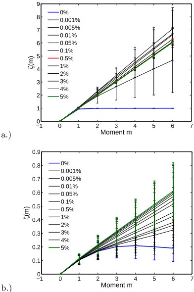
Figure 1 shows plots of the exponents ζ(m) Vs. m ob-tained from (3) by computing the gradients of logSm(τ) for (a) the L´evy process and (b) the multifractal model respectively. The exponents ζ(p) have been recomputed as outlying data points are successively removed, and we can see that removing a small fraction,∼0.001% of the
data leads to a large change in the computed ζ(p). A reliable estimate of the exponents from the data requires rapid convergence to robust values; shown in KCH to be a property of self-affine timeseries. We can see this be-haviour in the L´evy model which quickly converges to linear dependence ofζ(p) withpas expected.
a.)
−10 0 1 2 3 4 5 6 7 1 2 3 4 5 6 7 8 9 Moment m ζ (m) 0% 0.001% 0.005% 0.01% 0.05% 0.1% 0.5% 1% 2% 3% 4% 5% b.)
−10 0 1 2 3 4 5 6 7
[image:3.612.316.512.143.438.2]0.1 0.2 0.3 0.4 0.5 0.6 0.7 0.8 0.9 Moment m ζ (m) 0% 0.001% 0.005% 0.01% 0.05% 0.1% 0.5% 1% 2% 3% 4% 5%
Figure 1: ζ(m) Vs. mplots for a.) α= 1.0 symmetric L´evy process and b.) p= 0.6p-model process.
The multifractal p-model only begins to approach lin-earity after∼3% of the data is excluded. This apparent linearity in the p-model is actually a divergence in the values of theζ(p). We see this behaviour if we plot the value of one of the exponents from Figure 1 versus the percentage of points removed. This is shown forζ(2) for the L´evy process (upper panel) and thep-model (lower panel) in Figure 2. As we successively exclude outlying data points, the self-affine L´evy process quickly reaches a constant value for ζ(2) = 2/α = 2.0 whereas for the multifractal, the ζ(2) exponent shows a continuing sec-ular drift. Importantly, successively removing outlying data points does not convert the multifractal p-model timeseries into a self-affine process. In addition, a plot ofζ(p) versusp(Figure 1) is not sufficient to distinguish self-affine from multifractal behaviour, one also needs to examine the convergence properties of the exponents as outlying points are successively removed, as shown in Figure 2.
a.)
0 1 2 3 4 5
0.5 1 1.5 2 2.5
Percentage of pnts removed
ζ
(2)
[image:4.612.334.539.62.214.2]b.)
Figure 2: Exponent of the second momentζ(2) Vs. the per-centage of points excluded for a.) the L´evy model and b.) p-model.
a.)
−1 0 1 2 3 4 5 6
0.55 0.6 0.65 0.7 0.75 0.8 0.85 0.9 0.95
Percentage of pnts removed
ζ
(2)
WIND ACE
b.)
−1 0 1 2 3 4 5 6
0.65 0.7 0.75 0.8
Percentage of pnts removed
ζ
(2)
Figure 3: Exponent of the second momentζ(2) Vs. the per-centage of points excluded for a.) WIND and ACE at solar maximum and b.) WIND at solar minimum.
−1 0 1 2 3 4 5 6
0.4 0.45 0.5 0.55 0.6 0.65
ζ
(2)
percentage of removed points
Figure 4: Exponent of the second momentζ(2) Vs. the per-centage of points excluded for ULYSSES at solar minimum.
Figures 3a and b we plot ζ(2) versus the percentage of points removed inB2for intervals at solar maximum and
minimum respectively. Theζ values for these plots were obtained from an identified scaling range which spanned from ∼ 5.2 minutes to ∼ 2.7 hours (see e.g. [16, 22] ). Comparison of these plots with Figure 2 strongly suggests that at solar maximum, the magnetic energy density is self-affine; we can clearly identify a plateau with aH =ζ(2)/2 value ofH ≃0.44±0.02 for WIND andH ≃0.45±0.01 for ACE. At solar minimum, there is no clear plateau and the behaviour is reminiscent of the multifractal p-model. We have thus differentiated the distinct scaling behaviour at solar maximum and so-lar minimum. Intriguingly, it is at soso-lar maximum that we see self-similar behaviour; whereas at solar minimum the timeseries resembles a multifractal, reminiscent of in-termittent turbulence. Since the corona is complex and highly structured at solar maximum, this is highly sug-gestive that this self-similar signature in B2 is related
to coronal structure and dynamics rather than to local turbulence.
We can test this conjecture by considering observations of the solar wind where the coronal structure is maxi-mally ordered. We repeat the above analysis on a two month interval of ULYSSES data during solar minimum. The resulting plot of ζ(2) versus percentage of points excluded is shown in Figure 4. This plot again does not support self-affine scaling and is reminiscent of that of the p-model, strengthening previous results [15, 23]. Clearly, the behaviour ofB2 in the solar wind originating from
a corona dominated by ordered open field lines is not self-affine. The appearance of fractal versus multifractal behaviour in B2 is not a strong discriminator of
[image:4.612.70.266.398.678.2]4
speed is fast and uniform. We see fractal scaling in the ecliptic at maximum, where the average speed also alter-nates between fast and slow streams. Previous studies [23] have shown a variation with latitude and solar cycle of the level of multifractality of components of magnetic field. This may be related to the signature of the level of complexity in coronal magnetic structure which we have identified inB2 within the inertial range of turbulence,
but may also simply reflect a correlation with average so-lar wind speed. We have also verified that|B| does not show evidence of self-similarity for the intervals chosen for our study. More specifically|B|exhibits multifractal behaviour. This confirms the earlier results of Hnatet. al. [22].
The corona contains many long-lived structures which extend far out into the solar system mediated by the interplanetary solar wind [4]. At solar maximum these structures show a high degree of topological complexity. One model for these structures and their propagation is as a random walk or braiding of magnetic field lines with a measurable diffusion coefficient [2, 6, 24]. A diffusion process such as this intrinsically generates self-similar scaling, and may in a straightforward manner account for that shown here inB2at solar maximum. Alternatively,
the relevant process may be that of reconnection in the complex magnetic structure of the emerging coronal flux. Models for this include SOC based random networks [11] which again imply self-similar scaling. Our quantitative determination of the Hurst exponent H ≃ 0.45 of the self-affine scaling seen in the solar wind provides a strong constraint to these models.
The PDF resulting from such a self-similar process can be captured by a solution to a generalized Fokker-Planck equation (FPE) with power law scaling of the transport coefficients [17, 22]. Intriguingly, the associated Langevin equation transforms nonlinearly into that for a constant diffusion coefficient. The transformation may be equiva-lent to introducing a diffusion process with constant dif-fusion coefficient, on a space with non-Euclidean, self-similar, fractal geometry. This may provide a quanti-tative basis for models of transport of initially random fractal fields (the coronal source) in a turbulent flow (the solar wind). At solar minimum we see quite a differ-ent picture. Here the corona is topologically well or-dered magnetically. Thus in this case the fluctuations in B2 are dominated by the evolving turbulence of the
interplanetary solar wind which is well known to exhibit multifractal behaviour. Intriguingly, this self-affine sig-nature quantified here in B2 extends over the ∼ −5/3
exponent inertial range seen in the solar wind. This is at higher frequencies than the ∼1/f behaviour previously identified as a coronal signature in the solar wind [8]. Although models involving reconnection and flares and nanoflares have been proposed [25], estimates of the to-tal energy contained in such structures falls significantly short of that required for coronal heating [26]. Thus the
high-frequency self-similarity reported here may suggest further processes responsible for coronal heating.
We thank N. Watkins, M. Freeman and G. Rowlands for discussions. We acknowledge the PPARC for finan-cial support; R. P. Lepping and K. Oglivie for ACE and WIND data; and A. Balogh for the ULYSSES data.
∗ Electronic address: k.kiyani@warwick.ac.uk
[1] W. H. Matthaeus et. al., Phys. Rev. Lett. 95, 231101
(2005).
[2] J. Giacalone and J. R. Jokipii, The Astrophysical Journal
520, 204 (1999).
[3] C. J. Schrijveret. al., Nature394, 152 (1998).
[4] C.-Y. Tuet. al., Science308, 519 (2005).
[5] J. A. Klimchuk and L. J. Porter, Nature377, 131 (1995);
G. Vekstein and Y. Katsukawa, Astrophys. J.541, 1096
(2000).
[6] J. Giacalone, J. R. Jokipii, and W. H. Matthaeus, Astro-phys. J.641, L61 (2006).
[7] M. L. Goldstein, L. F. Burlaga, and W. H. Matthaeus, J. Geophys. Res.89, 3747 (1984).
[8] W. H. Matthaeus and M. L. Goldstein, Phys. Rev. Lett.
57, 495 (1986).
[9] M. J. Aschwandenet. al., Astrophys. J.535, 1047 (2000).
[10] E. T. Lu and R. J. Hamilton, Astrophys. J. 380, L89
(1991).
[11] D. Hughes, M. Paczuski, R. O. Dendy, P. Helander, and K. G. McClements, Phys. Rev. Lett.90, 131101 (2003).
[12] T. S. Horbury, M. A. Forman, and S. Oughton, Plasma Phys. Control. Fusion47, B703 (2005).
[13] C.-Y. Tu and E. Marsch, Space Sci. Rev. 73 (1995);
R. Bruno and V. Carbone, Living Rev. Solar Phys. 2
(2005).
[14] T. S. Horbury and A. Balogh, Nonlinear Processes in Geophysics4, 185 (1997).
[15] C. Pagel and A. Balogh, Nonlinear Processes in Geo-physics8, 313 (2001).
[16] B. Hnat, S. C. Chapman, G. Rowlands, N. W. Watkins, and W. M. Farrell, Geophys. Res. Lett.29(2002).
[17] B. Hnat, S. C. Chapman, and G. Rowlands, Physics of Plasmas11, 1326 (2004).
[18] K. Kiyani, S. C. Chapman, and B. Hnat, Phys. Rev. E
74, 051122 (2006).
[19] A. N. Kolmogorov, C. R. Acad. Sci. URSS30, 301 (1941).
[20] U. Frisch, Turbulence (Cambridge University Press, 1995).
[21] C. Meneveau and K. R. Sreenivasan, Phys. Rev. Lett.
59, 1424 (1987).
[22] B. Hnat, S. C. Chapman, and G. Rowlands, Phys. Rev. E67(2003).
[23] C. Pagel and A. Balogh, J. Geophys. Res. 107, 1178
(2002).
[24] L. M. Zelenyi and A. V. Milovanov, PHYS-USP47, 749
(2004).
[25] M. Velli, Plasma Phys. Control. Fusion45, A205 (2003).
[26] M. J. Aschwanden and C. E. Parnell, Astrophys. J.572,
1048 (2002).