Computationally Efficient Vision based Robot Control

(1)

COMPUTATIONALLY EFFICIENT

VISION-BASED ROBOT CONTROL

Matheus Terrivel

Master Thesis

December 2017

Examination Committee: Prof. dr. ir. M.J.G. Bekooij V. E. Hakim, MSc. Ir. J. (Hans) Scholten

Computer Architecture for Embedded Systems Group Faculty of Electrical Engineering, Mathematics and Computer Science University of Twente

7522 NH Enschede The Netherlands

(2)

Abstract

Video target tracking systems is a trending research topic, with a plethora of applications emerging from recent studies, with both visual object detection and tracking disciplines being the most notable, principally on embedded platforms. Not only are they employed in various fields, but also remarkably combines several branches of studies, such as control engineering, video processing, and more recently, machine learning and sensor fusion. Autonomous vehicles are a notable example, being equipped with a variety of sensors, including cameras, and widely apply image processing and sensor fusion techniques, thus providing more concise and high-level information, which increases robustness and more importantly, certainty, on decision making. However, such techniques must respect real-time constraints, especially in terms of timing, due the fact a delay might have a high cost under certain circumstances.

Currently, there is a broad interest in processing images with neural networks, which are superior in terms of performance and robustness in comparison to traditional image processing algorithms. Although the rapid development of image sensors in combination with neural network technology, computational power of the underlying platform is still a bottleneck, especially for embedded applications. Moreover, the platform is commonly responsible for multiple tasks, which might include a user interface, data processing, (digital) filtering and high-level control, thus cannot be fully dedicated to the neural network itself. Finally, modern system-on-chips comprise hardware accelerators and multiple processing cores, which enable embedded systems to accomplish the desired throughputs, and achieve better results and efficiency in comparison to pure software implementations. Most of the time, these SoCs are completely customizable and interaction between software and hardware is facilitated.

In this thesis, the focus is on both implementation and evaluation of a computational efficient robot control, based on neural networks to detect and localize a specific target (another robot), on an embedded platform. Sensor fusion and Kalman filtering are addressed, with the latter being used to post-process the output of the neural network, meanwhile the former combines encoder, accelerometer and gyroscope data which is used to derive the ego-motion information of the robot. Moreover, a specific approach for estimating the ego-motion impact in terms of pixels is proposed and discussed. The neural network, however, is not the focus, thus is only briefly discussed. During development, computational complexity, project extensibility and parallel tasks were the main concern, with the former being reduced whenever possible.

(3)

3

Acknowledgements

Initially, I would like to laud my supervisor, Professor Marco Bekooij, for providing me with his orientation, involvement and valuable feedback and monitoring throughout the development of my master thesis. Furthermore, the proposed project constantly provided new challenges, in addition to comprising different fields which regularly encouraged me to amass relevant knowledge and pushed me outside the comfort zone. Not only did I improve academically, but also personally, hence I am extremely grateful for this opportunity.

Next, I would like to thank all colleagues in both Robotics and Mechatronics (RaM) and Computer Architecture for Embedded Systems (CAES) groups, more specifically Viktorio El Hakim, Oğuz Meteer, Zhiyuan Wang, Konstantinos Fatseas, and Kiavash Mortezavi Matin, for every moment spent together, either by keeping me company, listening to silly problems, sharing a coffee, discussing scientific and personal topics, and providing relevant feedback during the development of this thesis.

Subsequently, not only am I grateful to each person I came across during my studies abroad, but also to every friend back in Brazil. Thanks to your cheering and encouragement to pursue and fulfill my aspirations, I was able to smoothly surpass countless adversities and finally achieve my goals.

Ultimately, I dedicate all work to my family, more specifically my father Geraldo José Domingues Terrível and my mother Rosária de Campos Teixeira, which supported me unconditionally during my studies. I own this achievement to you both, and hope you recognize that. Moreover, I wish my effort will be re-used in the future to impact peoples’ lives in a favorable manner.

Matheus Terrivel,

(4)

4

Glossary

Term Definition

0b__ Represents a binary value (usually an 8-bit value)

0x__ Represents a hexadecimal value (usually a 8 or 16-bit value)

ACK Acknowledge – In some communications when a message is sent, the receiver sends back an Acknowledge package to confirm that it received successfully the previous information

bps Bits per second – Refers to speed (i.e. baud rate) in a communication protocol C, C++, C# C, C plus plus and C sharp – Refers to programming languages

CRC Cyclic Redundancy Check – Algorithm used to perform error check when transmitting data

DC Direct Current

DoF Degree(s) of Freedom – Refers to how many degrees of freedom a device has EKF Extended Kalman Filter – Non-linear version of the Kalman Filter

fps Frames per second – Refers to camera frame rates

FPU Floating-Point Unit – Unit that is dedicated to floating-point arithmetic operations, usually a dedicated piece of hardware

GND Ground – Refers to ground or reference of a circuit

GPIO General-Purpose Input/Output, usually related to a microcontroller pin GPU Graphics Processing Unit – Refers to a graphic card

I/O Input/Output, normally refers to direction of a pin

I2C Inter-integrated Circuit – Intra-board communication protocol IC Integrated Circuit – Refers to a small chip

IMU Inertial Measurement Unit – Combination of motion sensors, usually a accelerometer, a gyroscope and a magnetometer

KF Kalman Filter – Optimal filter for linear systems, mainly used for data fusion LED Light-Emitting Diode – Electronic component which emits a light

LSB Least Significant Bit/Byte – Refers to ordination of bits/bytes MCU Microcontroller Unit

MSB Most Significant Bit/Byte – Refers to ordination of bits/bytes PC Personal Computer

PCB Printed Circuit Board

POSIX Portable Operating System Interface

PWM Pulse-width modulation – Modulation technique that sets an average voltage by switching on/off the voltage. Used for different kind of applications like RGB LEDs dimming

RMSE Root-Mean-Square Error – Measure of differences between values RPM Rotations Per Minute

RT Real-Time

SoC System-on-Chip – Refers to an integrated circuit which comprises components of a computer and other electronic systems

UART Universal Asynchronous Receiver/Transmitter – Serial protocol UI User interface

(5)

5

1. Introduction

Video target tracking systems have become a trend research topic, especially for embedded systems, covering several fields such as image, signal and video processing, machine learning, pattern recognition, and control engineering. Moreover, multiple sensors and thus sensor fusion techniques have been applied in order to improve the tracking performance [1]. Not only do vision tracking systems enable machines to perform complex tasks, but also require less hardware requirements and are easier to be implemented in comparison to other traditional systems, such as radar- or LiDAR-based systems. Thus, video target tracking is widely applied in commercial applications, ranging from medical to autonomous vehicles. Whenever multiple sensors are used, sensor fusion techniques are used in order to derive relevant information and improve the overall performance of the system, with the Kalman filter and its variations being the most commonly used.

In terms of target detection and localization, the state-of-the-art techniques are based on neural networks, which have been replacing traditional image processing techniques due to their superior performance and robustness. However, neural networks are computationally expensive and other technologies are still utilized for object detection in embedded systems, such as radar, due the fact data processing is faster, thus real-time processing is possible. In terms of sensors, most video target tracking systems comprise cheap and accurate inertial measurement units (IMUs), in addition to (mono- or stereo-)cameras, mainly focusing on improving the tracking algorithm and performing Simultaneous Localization and Mapping (SLAM). However, multiple sensors increase overall complexity of the system, which must include sensor fusion techniques, hence requires even more resources from the underlying platform.

The rapid development of image sensors enables stable streams with high framerate and image quality, easily achieving 60 fps at 1080p or higher resolution, which contribute to increasing the target recognition, especially for neural network-based implementations. Moreover, advances on sensor technologies provide lightweight and more accurate devices. Over the last decade, however, most video tracking systems had been implemented on a remote computer or cluster, equipped with high performance CPUs and GPUs, specifically addressing the computational complexity issue of both image processing and sensor fusion techniques. The remote device then transmits back commands to the embedded platform, which introduces latency for (mobile) applications, decreasing their performance because real-time requirements cannot be guaranteed. Moreover, standard computers are not power-efficient, expensive and relatively large, hence not feasible for mobile applications.

More recently, several system-on-chips significantly improved their hardware capabilities, enabling data processing to be performed in the embedded platform itself, as the hardware conditions do not represent a bottleneck to implementing complex video processing and sensor fusion algorithms. Considering such SoCs comprise hardware accelerators and multiple processing cores, being most of the time completely customizable and simplifying interaction between software and hardware, embedded systems are capable of achieving the desired throughputs, achieving better results and efficiency in comparison to pure software implementations.

(8)

8

such as a dual-role HDMI port, and supports bare-metal code, alongside embedded Linux and hardware accelerators. Hence, the focus of this thesis is to implement and evaluate a video tracking system with object recognition and tracking, which exploits both the FPGA fabric for executing the neural network – the most computationally expensive part of the application –, and the ARM Cortex-A9 for data fusion and high-level control. The application is a toy example, and its goal is to not only track a specific target, but also follow it by means of controlling another robotic platform equipped with sensors and actuators. This thesis summarizes and describes the whole design process and decisions during the development of such system, except the neural network hardware implementation. More specifically, due to the fact the neural network in the end of this project was still not ported to the FPGA, a PC was used instead. However, decisions during the project were made taking into account the underlying platform would be an embedded system with limited resources, thus the final implementation can be easily ported to the ZYBO board, for instance.

This chapter introduces the research problem: initially, the problem is explained in more detail and the major research objectives are defined; subsequently, the contributions of this thesis are presented and briefly discussed, followed by the outline of this report in the last section.

1.1 Problem definition

Porting a visual tracking system that comprises both tracking with a neural network and sensor fusion is not an easy task. A pure software solution demands vast computational capabilities, with the neural network being extremely computationally intensive due the required operations performed on the frames. A pure hardware solution, on the other hand, is limited by the amount of resources available, and is commonly limited in terms of flexibility and configurations. Recent solutions utilize multiple sensors and complex sensor fusion techniques in order to navigate, instead of perform tracking, such as SLAM [4], Extended Kalman Filters [5, 6, 7, 8], Unscented Kalman Filters [8, 9, 10], among others, in addition to some combining different techniques [5, 6, 9] which demands even more resources, thus computational power. Camera-IMU setups are widely applied for positioning [10, 11], which requires online camera external parameters calibration, performed by Kalman filters. Neural networks are rarely used in mobile applications due its complexity and execution time which restrains real-time requirements, with either traditional image processing techniques being applied instead, or third-party libraries used, such as skeleton tracking [4], for instance. Moreover, whenever a neural network is indeed utilized for object detection and tracking, it is executed in a remote PC [12], and filtering its output is rarely implemented, which greatly degrades the performance in occlusion scenarios [4] or false-negatives. Instead, Kalman filters usually are applied to pre-process data which is inputted to the neural network [13, 14].

Considering the aforementioned facts, this thesis addresses an alternative solution in order to detect and localize an object with a neural network, taking into account the ego-motion impact and filtering the output of the neural network with a robust filtering technique, in order to properly steer a robot and follow a target, all implemented in a resource-constrained embedded system. Moreover, this thesis stresses the following objectives:

1. Implement a low-level system which is responsible for sensor fusing data and steering a robot: a. Using a resource-constrained embedded system;

(9)

9

c. Improving the refresh rate of the ego-motion data; d. Properly controlling the speed;

e. Providing ego-motion data to a higher-level system. 2. Realize a robust visual object tracking system:

a. Using software which interacts with hardware in a resource-constrained embedded system;

b. Using a neural network-based detection and localization implementation, ideally on hardware – implementation of the neural network is NOT addressed, however; c. Coupling a Kalman filter to improve stability and addressing both tracking with

occlusion and possible false negatives outputted by the neural network; d. Retrieving ego-motion data from the lower-level system;

e. Considering the ego-motion impact on the target being tracked, in pixel speeds; f. Interacting with the low-level system in order to follow the target.

3. Analyze and evaluate the complete system: a. Considering delays;

b. Identifying bottlenecks; 4. Test the complete system in practice.

In summary, the research questions are as follows: Is it possible to implement application which comprises tracking and sensor fusion techniques on a practical embedded system? Furthermore, what are the complications for such system?

1.2 Contributions

In summary, this thesis contributes to five major points. Initially, it (1) addresses the usage of a complementary filter to fuse encoder and IMU data, more specifically accelerometer and gyroscope information. Not only does such filter reduces computational complexity, but also boosts the ego-motion speed accuracy and refresh rate, being particularly useful when low-cost and low-accuracy sensors are deployed, although this technique is currently not often applied.

Secondly, the ego-motion, more specifically speed and angular velocity with respect to heading, is considered and its impact on the object being tracked is estimated by a simpler (but specific) method, which does not require computationally expensive algorithms (2). The output of the neural network applied for detection and localization is additionally filtered by standard Kalman filters, which are based on a linear model and their implementation do not depend on matrix operations, reducing even further the require computational power of the underlying platform (3). Moreover, the derived ego-motion impact is used by the Kalman filters, making it possible to keep tracking the target when occlusions occur, in addition to common false-negatives outputted by the neural network (4).

Finally, distance control is abstracted by investigating pixel control instead, hence complex translations between camera and world coordinates are avoided (5). Furthermore, two PID controllers are combined in order to simplify steering the robot.

(10)

10

from different areas. Hence, the implementation is a complete base system in terms of structure, hardware and software, which can be applied in a variety of applications.

1.3 Thesis outline

Heretofore, the topic of this thesis and related research has been introduced. In the upcoming chapters, the whole system is extensively discussed, with its complete overview being depicted in Figure 1 below:

Figure 1. Complete system overview

Chapter 2 describes the robotic system (highlighted in red), by introducing the overall structure, the related embedded hardware, improvements done to the standard libraries, followed by the complementary filter used for fusing encoder and IMU data and the respective results. Finally, the protocol used for communicating with this system is discussed and the final implementation detailed.

Chapter 3 is the unit of this thesis, and addresses the tracking system (highlighted in black), briefly introducing the camera used and the neural network scheme. Subsequently, the Pre-Kalman filter module is detailed, which is responsible for translating the ego-motion impact to pixel speeds which are forwarded to the Kalman filter. The Kalman filter used for filtering the output of the neural network is then assessed, regarding its design and additional algorithms applied specifically for tracking, alongside the obtained results. Subsequently, the Pixel Control module is presented and explained, which is responsible for computing the speed and direction that must be forwarded to the robotic system in order to it properly follow the target. Finally, the final implementation in terms of both hardware and software related to the tracking system is explored, including the drivers developed for the Kalman filters, PID controllers and communication with the robotic system.

Chapter 4 analyzes the complete system behavior, exploring the impact of the delay on the performance, alongside a basic dataflow graph discussion to explore RT analysis techniques.

(11)

11

2. Robotic system

Figure 2. Robotic system outline

In order to introduce the complementary filter, which is the first main part of this project, the underlying robotic system used – the Makeblock Ultimate Robot Kit V2.0 10-in-1 [15] -, with its mechanical structure, key hardware modules likewise extra ones and their capabilities, are briefly discussed. Moreover, improvements with respect to the default software libraries are assessed, considering the desired functionalities of the complementary filter itself in addition to overall improvements, such as the low-level speed controller. Finally, the filter is explained and analyzed, alongside the micro-protocol used for communicating with the robotic system, as well as the final architecture in terms of both software and hardware. In summary, the highlighted blocks shown in Figure 2 above are detailed in the upcoming sections.

The Makeblock Ultimate Robot Kit has many structural parts, a mainboard – the MegaPi -, Bluetooth connectivity and several (proprietary) modules. This kit was readily available in the beginning of the project and comprised, among others, an Inertial Measuring Unit (IMU) module, DC motors coupled with encoders, and their respective drivers, which are required for the final application: follow an object. Moreover, it is simple to use and tailor to this application, without much effort. All

development tools are provided in the seller’s website, and the system can be fully customized by the

user, in terms of software and structure. Hardware components, on the other hand, are complete modules and is up to the user to integrate them or not. For a detailed description, one should refer to [15].

Although the complementary filter will be extensively discussed later in this chapter, it is important to define its inputs and outputs briefly due the fact most design decisions were based on what it requires for the desired behavior. In summary, the complementary filter is used to improve and complement the speed estimation procedure, and fuses data from both encoder and accelerometer, which is relevant for the tracking system. Moreover, the tracking system requires data from a gyroscope, but this will be further explored in Chapter 3. Taking this into consideration, the complementary filter’s

(12)

12

and the linear speed derived with the encoder. The output, on the other hand, is the fused linear speed, with the gyroscope data being directly forwarded to the tracking system.

Furthermore, a set of basic requirements and functionalities was defined for the robotic system, which should follow another robot, and thus must be able to:

• Move forwards, backwards, and turn;

• Support a camera on top: the frames will be further processed by the tracking system; • Process data from an IMU: necessary for the complementary filter;

• Control the speed of the motors: low-level speed control; • Receive speed references from the tracking system;

• Send relevant data to the tracking system: current speed and angular velocities.

2.1 Structure

The kit used in this project has several mechanical parts, such as plastic gears, acrylic supports, screws, and metal part, which can be assembled in different ways. Although there are default configurations

provided by the seller alongside the respective piece of software, such as “Robotic Arm Tank”, “Self

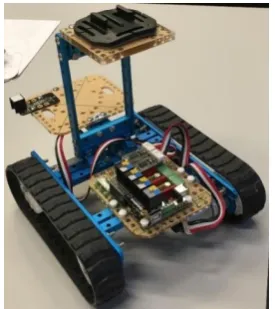
[image:12.595.229.367.416.571.2]

-Balancing Robot” and “Robotic Bartender” [15], for this project a custom setup was built which contemplates a base structure with two tracks driven by two separate DC motors, and two elevated platforms: a shorter one for supporting the battery, and a taller one to accommodate the camera. Finally, a support for the main board is required and should be located as close as possible to the modules used. The structure used is shown in Figure 3 below:

Figure 3. Robotic system structure

The tracks have been utilized due the fact driving the robot in a different manner would overcomplicate its odometry model and drive procedure, especially when changing direction. Not only do the tracks simplifies the operation, but also improves robustness due the fact they overcome obstacles easier. Furthermore, this structure complies with the previous requirements:

• Move forwards, backwards, and turn: with tracks and two separate motors, the robot can be steered properly;

• Support a camera on top.

(13)

13

2.2 Embedded hardware

Besides the mechanical parts, the kit includes a microcontroller board based on ATmega2560 [16] –

the MegaPi, which is both Raspberry Pi and Arduino compatible. Programming is done through USB, and for this application only the Arduino IDE was necessary during development, although it is possible to use different development tools. Moreover, the kit comprises several electronic modules which are plug-and-play, with the most relevant ones being: Bluetooth, DC motor driver, ultrasonic sensor, RJ25 shield for I2C/UART modules, 3-axis accelerometer and gyroscope sensor, and a compass. In total, three (3) encoder motors are also included, apart from the aforementioned modules, which are DC motors coupled with encoders. Cables are provided and connections are simple to use, thus will not be explained in this section. The complete parts list can be found in [15].

With respect to hardware requirements, the system must support, at least: • Driving 2 DC motors simultaneously;

• IMU connection for the complementary filter;

• Serial communication or (optimally) wireless module for exchanging data with a master and debugging;

• Floating-point operations for control loops, filtering and data processing.

2.2.1 MegaPi board

The MegaPi, as explained before, is based on the ATmega2560 microcontroller and can drive up to 10 servo motors, 8 DC or 4 stepper motors simultaneously. Additionally, most I/O pins are exposed and can be used for custom hardware and software implementations, as depicted in Figure 4 below. Note

that the motors’ circuitry is highlighted in purple, power input and switch in gray, Bluetooth in orange

and the microcontroller itself in yellow.

Figure 4. MegaPi board, with highlighted relevant parts

For this project, the MegaPi board and modules are sufficient and meets the requirements: • DC motors: it is capable of driving up to 4 simultaneously;

• IMU: a 3-axis accelerometer and gyroscope sensor are included in the kit;

(14)

14

Although the ATmega2560 is an 8-bit microcontroller, it has software support for floating-point operations which are typically fast (< 1 milliseconds for division), and commonly used for control loops and filtering techniques. Taking into consideration that both the complementary filter and data processing (for the IMU) are simple and do not require many calculations, this platform is capable of performing the necessary operations on time.

Finally, it is important to note that this board operates at 5V, and its power-in range must be between 6-12V, in case a battery is used. The complete specifications of the board and ATmega2560 can be found in [15] and [16], respectively. In terms of software, the MegaPi has a complete open-source library, available at [17]

2.2.2 Sensors & Actuators

Before defining and integrating all components, it is important to consider both the available sensors and actuators. Despite that several electronic modules are included in the kit, only few are required for the application:

• IMU unit, more specifically an accelerometer and a gyroscope, for the complementary filter; • DC motors for movement;

• DC motor drivers;

• Encoders for speed control;

• Wireless module for communication: optional, as a wired connection is more reliable.

This section describes the motors used, alongside the feedback sensors necessary for speed control and finally the IMU required by the complementary filter.

Encoder motors

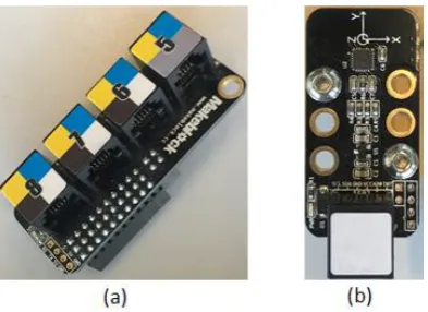
In total the kit includes three (3) 25mm encoder motors, which are DC motors coupled with an incremental encoder: all three operate at 9V, but only two can achieve a higher speed (185 RPM ±10%) with the other being slower (86 RPM ±10%). The latter, however, has a higher torque in comparison to the former, and is typically used for lifting a robotic arm, which is not the case for this application. Thus, both identical encoder motors are used for driving the robot, one on each side. The encoder motor is depicted in Figure 5a below, with the encoder being in the back, close to the proprietary connection. Other specifications can be found in [18].

Figure 5. Encoder motor (a) and its driver (b)

(15)

15

different ways – coasting (free rotation) or braking – and its rotation direction can also be determined. Fortunately, the kit also provides the driver module for the encoder motors, which is shown in Figure 5b above, and must be place in either slot 1 or 2 of MegaPi (check Figure 4). Moreover, the encoder connections are properly routed to the microcontroller pins in order to derive the speed.

[image:15.595.206.389.364.451.2]

There are different ways of keeping track of a motor’s RPM, with tachometers and hall-effect sensors being an example. However, when considering all aspects of each technology, quadrature incremental or absolute encoders stand apart due their price, size, availability, and reliability. Not only do encoders require less mechanical components, but also are easy to mount and require simple data processing. A quadrature relative or incremental encoder measures a change in position, and usually outputs two channels (A and B – the quadrature signals) and one index pulse (X). The former signals are toggled in a certain order depending on the rotation direction (clockwise or counter-clockwise), and the latter is pulsed once every complete revolution (Figure 6). The amount of pulses per revolution (PPR) outputted by a one channel is stated in the datasheet, thus rotations per second can easily be derived and converted (e.g. to Hz, RPM) either from the two output channels, or from the index pulse itself by measuring the time between one or several pulses, which is less accurate (i.e. integer number of revolutions). Hence, such encoder provides rotational velocity, direction, and relative position feedback, and one per motor is required.

Figure 6. Quadrature signals and index for counter-clockwise rotation (a), outputted by the incremental encoder (b)

Although the encoder motor already includes an incremental encoder, no datasheet is provided by the supplier. This is not a problem, as by visually inspection it is possible to determine it is a low-quality device with 8 PPR, thus low resolution, which negatively impacts the speed control. However, the supplier does provide the necessary drivers [3] to derive the RPM and no extra hardware nor mechanical parts are needed. With respect to software, the “MeEncoderOnBoard” driver is used for

initializing, configuring, and utilizing the encoder motors. Check Appendix C: Embedded Software for further details.

IMU

(16)

16

[image:16.595.201.398.162.305.2]

One of the modules included in the kit is a 3-axis accelerometer and gyroscope (Figure 7b), which has been and will be referred to an IMU throughout this document, even though the magnetometer is not involved. Moreover, the application only requires data from an accelerometer and gyroscope, with the former being used to determine the linear speed, meanwhile data from the latter is directly forwarded to the tracking system. Hence, the magnetometer will not be discussed in this section.

Figure 7. RJ25 shield (a), and 3-axis accelerometer and gyroscope module (b)

The module shown in Figure 7b above is an I2C device and both accelerometer and gyroscope full-scale ranges are programmable, with the core IC being the MPU6050 – full specifications can be found in [19]. Moreover, the module uses a RJ25 connector and must be correctly connected to the MegaPi board through the RJ25 shield (Figure 7a). Note that the module has a white label on top of its connector, which must match one of the colors on top of the RJ25 shield. In this case, it should be connected to connector number 6, 7 or 8. Usage is straight forward with respect to software, which

depends only on the “MeGyro” driver for initializing, configuring, and utilizing the encoder motors –

Check Appendix C: Embedded Software for further details.

2.3 Library improvements

The processing board and its compatible modules work out-of-the box with the open-source library provided [3]. More specifically for this application, however, two drivers are used:

“MeEncoderOnBoard” and “MeGyro”, which handle the encoder motors and the IMU module,

respectively. By exploring the source code of both libraries, one may find points of improvement, or customize it in order to add specific functionalities, for instance. The former relates to a problem found in the speed control, and the latter to instability issues and a lack of flexibility with the data retrieved from the IMU module. The main goal of modifying such drivers is to improve the overall behavior, robustness and stability of the robotic system, and in this section the major modifications are presented, further explained and justified.

2.3.1 Speed Controller

The first issue addressed is the speed controller provided by the “MeEncoderOnBoard” driver, which

(17)

17

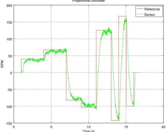
according to the documentation. It is important to notice that the reference must always be provided in RPM, and in this scenario the same speed is provided for both encoder motors. Initially, however, both sides were tested and presented highly similarities, thus the upcoming results depict one side only. Two metrics are used to compare the performance: the settling time for 95%, and the root-mean-square error (RMSE), with the latter being computed with the following formula:

𝑅𝑀𝑆𝐸 = √1

𝑁∗ ∑(𝑟𝑒𝑓𝑒𝑟𝑒𝑛𝑐𝑒𝑖− 𝑠𝑒𝑛𝑠𝑜𝑟𝑖)

2 𝑁

𝑖=1

(2.1)

[image:17.595.156.435.281.503.2]

The performance is shown in Figure 8 below, with the reference depicted in red and the actual sensor (i.e. encoder) readings in green.

Figure 8. Proportional controller response

(18)

[image:18.595.162.436.72.298.2]

18

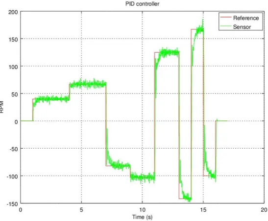
Figure 9. PID controller response

In this setup, the proportional (𝐾𝑝), integral (𝑇𝑖) and derivative (𝑇𝑑) gains were tuned to 1.7, 0.1 and

0.0001, respectively, and the sampling frequency was increased to 50 Hz. With such configuration, the settling time was reduced to 0.3 second, corresponding to a reduction of 62.5% in comparison to the original controller. Moreover, overshoots do not surpass 5% of the reference value, and the RMSE was decreased to 27.86 RPM (55.83% reduction). The oscillation in the steady state will be further addressed by the complementary filter, which outputs a more stable speed value. Additional information about the PID controller, its implementation and tuning procedure can be found in Appendix A: PID Controller.

2.3.2 IMU

The IMU library is called “MeGyro”, although is comprises both an accelerometer and a gyroscope.

During initial tests with the module, a few drawbacks were discovered:

• The calibration procedure did not take into consideration the accelerometer offsets (advised in the datasheet [19]);

• The driver only outputted fused (with a complementary filter) gyroscope data: yaw, roll and

pitch. Hence the name “MeGyro”;

• The driver only outputted processed data – raw data from the sensors could not be retrieved. Note that raw data corresponds to integer values directly retrieved from the sensors, meanwhile processed considers both offset and sensitivity, resulting in a meaningful value and unit (i.e. m/s2_{and °/s);}

• If the module was placed nearby metal parts, the system would often halt during initialization due magnetic interferences.

(19)

19

requests processed data from the driver, by simply deducting the offsets from the raw readings. Note that calibration is always performed upon startup, thus the robotic system must always be in a flat surface and not be disturbed during initialization, otherwise behavior might be unpredictable due to wrong readings.

As the complementary filter input requires a speed value derived from the IMU, it is necessary to make the accelerometer data available in addition to the gyroscope data, which will further be used to calculate the speed. Additionally, it is rather advantageous to provide both raw and processed data retrieved from the sensors for debugging purposes. These modifications were both addressed simultaneously, by including specific functions to the library. Due the fact unique methods were added, usage of this driver is different from the original version. For more details, one should refer to Appendix C: Embedded Software.

Data signaling depends on how the module is placed with respect to the robot, and will be discussed in the end of this chapter. It is extremely important to keep the module away from metal parts and motors, and ideally it should be placed on top of an acrylic platform. Otherwise, the robotic system will most likely malfunction due to interferences and halt during initialization.

Finally, the accelerometer and gyroscope sensitivities were set to 2g and 500 °/s, respectively. The former corresponds to the highest resolution, and was used due the fact the linear accelerations are as precise as possible, which decreases errors for the following speed estimation step. The gyroscope sensitivity, on the other hand, can be further decreased to 250 °/s which corresponds to the best resolution, but it is not required for this application: based on tests, the robotic system is not capable of turning faster than 360 °/s. Furthermore, both sensitivities constrain the sampling frequency, and for this specific configuration up to 1kHz can be achieved. This is enough for both complementary filter and tracking system (most likely running below 200Hz). The former benefits from this high sampling frequency, as currently bottleneck the sampling frequency for the speed is restrained by the encoder readings.

2.4 Complementary Filter

Estimating the ego-motion of the robotic system is an important part of the application, considering such information will be further used by the Kalman filter and directly impacts the overall performance. Thus, being able to estimate the speed as precise and fast as possible is required. One might assume the encoder readings are enough, but in fact it only updates the readings at 50Hz, with the software improvements previously discussed. The IMU readings, on the other hand, are considerably faster for the presented sensitivities: 1kHz. Hence, by fusing both sensor data it is possible to achieve a sampling frequency of 1kHz in a low-cost platform.

(20)

20

original implementation of the IMU module (“MeGyro” driver) utilized a complementary filter to fuse

accelerometer and gyroscope data and output less noisy and more accurate angular speeds (i.e. yaw, roll and pitch). Such technique is widely used for this type of sensor fusion, with many practical examples found in literature [21, 22, 23]. Furthermore, other applications use the same technique but the interest is specifically on estimating heading (i.e. yaw) and attitude [24, 25]. In summary, the complementary filter enhances accuracy, increases the sampling frequency, reduces complexity, and can be implemented in a low-cost platform as well. Hence, this section further explores the complementary filter (1st_{and 2}nd_{order), addresses the necessary speed estimation techniques, and}

finally presents comparisons and results.

2.4.1 Filter structures

The 1st_{order complementary filter corresponds to two filters in parallel, with the same cut-off}

frequency: a high-pass and a low-pass filter. Moreover, the filter’s name corresponds to the relations

between both high- and low-pass filter gains, which are complementary: 𝐺𝐻𝑃𝐹+ 𝐺𝐿𝑃𝐹= 1. The

general structure of the 1st_{order complementary filter for the robotic system is depicted in Figure 10}

below.

Figure 10. First-order Complementary Filter

The generic implementation of the 1st_{order complementary filter is straight-forward:}

𝑜𝑢𝑡𝑛= 𝐾 ∗ 𝑖𝑛𝑝𝑢𝑡_1𝑛+ (1 − 𝐾) ∗ 𝑖𝑛𝑝𝑢𝑡_2𝑛 (2.2)

𝐾 = 𝑓𝑐 (𝑇𝑠+ 𝑓𝑐)

(2.3)

With 𝐾 being the time constant, 𝑓𝑐 the cut-off frequency, and 𝑇𝑠 the sampling period. The timing

constant can be interpreted as a boundary between trusting one reading and the other, being usually tuned in practice, even though there are methods in literature to calculate it [23]. Note that 𝐾 can be computed on-the-fly, if the 𝑇𝑠 (or 𝑓𝑠) is correctly measured and the cut-off frequency is known a priori.

However, 𝑓𝑐 is commonly unknown thus 𝐾 is defined or computed offline. The high-pass filter gain

corresponds to 𝐾 itself, meanwhile the low-pass filter gain is the complement: 𝐾 − 1. Thus, both inputs must be carefully selected to match the desired filters.

(21)

21

constant is not computed dynamically, but defined as a constant, and by considering all the aforementioned information, (2) becomes:

𝑣𝑓= 𝐾 ∗ 𝑣𝐼𝑀𝑈+ (1 − 𝐾) ∗ 𝑣𝑒𝑛𝑐 (2.4)

With 𝑣𝑓 being the fused speed, 𝑣𝐼𝑀𝑈 the speed derived from the IMU, and 𝑣𝑒𝑛𝑐 the speed derived

from the encoder.

A 2nd_{order complementary filter might be implemented as well, because it theoretically yields a better}

result at a cost of a more complex structure [23, 25], which involves two integrations as shown in Figure 11 below.

Figure 11. Second-order Complementary Filter

Note that 𝐾1 and 𝐾2 are positive gains, typically tuned in practice, and can be related as follows to

simply work with a single gain 𝐾:

𝐾1= 2 ∗ 𝐾 (2.5)

𝐾2= 𝐾2 (2.6)

Implementation is more complex, and can be divided into intermediate steps. Based on Figure 11, one might use the following equations to realize the 2nd_{order complementary filter:}

𝐴𝑛 = 𝑖𝑛𝑝𝑢𝑡_2𝑛− 𝑜𝑢𝑡𝑛−1 (2.7)

𝐵1 = 𝐴𝑛∗ 2 ∗ 𝐾 (2.8)

𝐵_2𝑛= 𝐴𝑛∗ 𝑇𝑠∗ 𝐾2+ 𝐵_2𝑛−1 (2.9)

𝐶𝑛= 𝐵1+ 𝐵_2𝑛+ 𝑖𝑛𝑝𝑢𝑡_1𝑛 (2.10)

𝑜𝑢𝑡𝑛= 𝐶𝑛∗ 𝑇𝑠+ 𝑜𝑢𝑡𝑛−1 (2.11)

For this application, (2.7), (2.10) and (2.11) become:

(22)

22

𝐶𝑛 = 𝐵1+ 𝐵_2𝑛+ 𝑣_{𝐼𝑀𝑈𝑛} (2.13)

𝑣_𝑓𝑛= 𝐶𝑛∗ 𝑇𝑠+ 𝑣_𝑓𝑛−1 (2.14)

It is important to notice that regardless the filter order, an integration method must be implemented to estimate the speed, which will be addressed in the next section. Obviously, both inputs must be provided in the same unit and in this case, meters/second was used.

2.4.2 Speed Estimation

Integration is strictly related to the complementary filter, due the fact a typical 1st_order

implementation requires so. More specifically, the accelerometer provides 3-axis linear accelerations which must be integrated to derive the speed, as follows:

𝑣(𝑡) = ∫ 𝑎(𝑡)𝑑𝑡

𝑡

0

(2.15)

With 𝑣(𝑡) being the linear speed, and 𝑎(𝑡) the linear acceleration, for a single axis. Notice that integration is related to continuous time, but the system is digital, thus a summation is used for the implementation. In this case, the speed at moment 𝑛 is computed by summing the previous speed (𝑣𝑛= 0, 𝑛 < 0) and the value retrieved with an approximation rule, being generalized as follows:

𝑣𝑛= 𝑣𝑛−1+ {𝑎𝑝𝑝𝑟𝑜𝑥𝑖𝑚𝑎𝑡𝑖𝑜𝑛 𝑟𝑢𝑙𝑒} (2.16)

Although there are many ways of estimating the speed in a robotic system, in this setup the procedure was purely encoder based. Such method delivers fairly accurate results, basically dependent on the encoder resolution itself and does not require an integration method for computing the speed, but may be improved by sensor fusing the IMU data that, on the other hand, does need an integration procedure. Furthermore, the interest is in estimating a 1D speed for this application, that basically corresponds to a forward or backward movement due to the robot's constraints (tracks): it can neither move sideways or up/down. Although the robot might be yawing, rolling or pitching, only the latter affects the 1D speed component. This section discusses optional approaches for speed estimation, considering the available hardware and computational capabilities of the underlying platform.

Accelerometer based

As previously stated, 3-axis linear accelerations are retrieved from the accelerometer, in m/s2_{, and in}

order to estimate the speed an (digital) integration method must be implemented. Moreover, the accelerometer should be correctly calibrated for its static linear accelerations (offset), and go through the following procedures [26] in order to yield reasonable results:

1. Low-pass filter for noise reduction;

2. Window-filter for mechanical noise reduction;

3. Movement-end check to force the integration to 0, when the system has stopped.

(23)

23

for estimating the speed is depicted in Figure 12 below. Due the fact the offsets are computed during the IMU initialization and automatically used when processed data is requested, the low-pass filter procedure for noise reduction is initially addressed. Reducing the noise is critical in order to decrease major errors during the integration procedure, which is performed by both the low-pass and window filters [26].

Figure 12. Accelerometer-based speed estimation procedure

One of the simplest implementations of a low-pass filter in digital systems is averaging: high-frequency disturbances are filtered out. However, simple averaging adds unnecessary delay to the system, as at least 𝑁 samples must be averaged before outputting a filtered value. There are alternatives that specifically address this issue, such as the moving average: the output is computed whenever a sample is retrieved by averaging it with the previous 𝑁 − 1 samples. Notice, however, that this method still comprises a delay of 𝑁 samples, but only during initialization. Another issue of the moving average (and simple average) is the division, which is computationally expensive. The exponential moving average (EMA) is then introduced, which yields surprisingly similar results with respect to the moving average, does not require division operations and is simpler to implement. Taking these factors into consideration, alongside the underlying platform, the EMA was chosen to be implemented. The EMA for a single sample is computed as follows:

𝑜𝑢𝑡𝑛 = 𝛼 ∗ 𝑖𝑛𝑝𝑢𝑡𝑛+ (1 − 𝛼) ∗ 𝑜𝑢𝑡𝑛−1 (2.17)

𝛼 = 2

(𝑁 + 1) (2.18)

With 𝛼 being defined based on the filter order 𝑁, thus can be computed a priori. Setting 𝑁 to a high value can result in a loss of data, meanwhile setting it to a low can result in an inaccurate output value. The exponential behavior corresponds to the (1 − 𝛼) factor which is multiplied by the previous output 𝑜𝑢𝑡𝑛−1, differently from the moving average that considers the previous input values instead.

(24)

24

Figure 13. EMA sample responses for different N values

With respect to this application, the best results for the accelerometer readings were obtained with 𝑁 = 3 during testing, hence (2.17) becomes:

𝑓𝑖𝑙𝑡𝑒𝑟𝑒𝑑 𝑎𝑐𝑐𝑛= 0.5 ∗ (𝑎𝑐𝑐𝑛+ 𝑓𝑖𝑙𝑡𝑒𝑟𝑒𝑑 𝑎𝑐𝑐𝑛−1) (2.19)

Next step is to implement a window-filter to reduce mechanical noise, as minor errors in acceleration could be interpreted as a constant velocity and will be summed [26]. Moreover, the low-pass filter might produce residual erroneous data, so a window of discrimination between valid and invalid data and for the no-movement condition must be implemented [26]. Implementation is straight forward: if the input is within the maximum and minimum window values, the output is 0; otherwise, the output is the input. A sample behavior of the window-filter is depicted in Figure 14 below, where the maximum and minimum window values are set to ±0.3, respectively:

Figure 14. Window-filter sample response

(25)

25

With the accelerometer readings properly pre-processed with both low-pass and window filters, the linear speed can finally be estimated through an integration method. A common approach is to utilize the 1st_{order trapezoidal rule, that approximates an integral by accumulating the area of several}

trapezoids, as shown in Figure 15 below.

Figure 15. Illustration of the trapezoidal method

Formally, the trapezoidal rule is defined for continuous time as follows:

∫ 𝑓(𝑥) 𝑑𝑥 ≈ (𝑏 − 𝑎) ∗ (𝑓(𝑎) − 𝑓(𝑏)

2 )

𝑏

𝑎

(2.20)

For discrete time and considering the application, however, (2.20) reduces to the following formula which is derived from both the trapezoidal rule combined with (2.16):

𝑣𝑛= 𝑣𝑛−1+

(𝑎𝑐𝑐𝑛+ 𝑎𝑐𝑐𝑛−1) ∗ ∆𝑡

2 (2.21)

With 𝑣𝑛 being the speed estimation, 𝑎𝑐𝑐𝑛 the linear acceleration, and ∆𝑡 the sampling time for

sample 𝑛. Not only does the trapezoidal rule greatly reduce integration error, but it has a simple implementation and requires a single floating-point multiplication, hence this method was chosen for speed estimation.

(26)

26

After several tests, the maximum quantity of consecutive readings allowed before forcing the speed to zero was set to 25.

Encoder based

Deriving the speed with the encoder is a simpler matter, due the fact the sensor’s output signals are

captured by the microcontroller, with the library handling the conversion from PPR to RPM, as previously discussed. However, the robotic system uses two encoder motors to move around, and information from both encoders must be properly combined, which result in a 1D speed as required. Thus, encoder-based speed estimation is reduced to standard odometry of the robotic system.

Due the fact there is no interest in performing dead-reckoning, neither heading or position are estimated and using a partial-odometry is enough for the application. Considering the simplistic robotic system structure, a basic model was derived based on [27, 28, 29, 30, 31] in which slippage is not considered [32]. In this scenario, the combined encoder speed 𝑣𝑒𝑛𝑐 is the mean of the encoder

readings from both sides:

𝑣𝑒𝑛𝑐 =

𝑣𝑅+ 𝑣𝐿

2 (2.22)

With 𝑣𝑅 and 𝑣𝐿 being the right and left encoder readings, respectively, in RPM. Alternatively, one

might compute the velocity of each encoder motor, in meters per second, based on the wheel’s radius

𝑅, encoder’s resolution 𝑃𝑃𝑅, pulse difference ∆𝑝𝑢𝑙𝑠𝑒𝑠 and time between measurements ∆𝑡, as follows:

𝑣 =2 ∗ 𝜋 ∗ 𝑅 ∗ ∆𝑝𝑢𝑙𝑠𝑒𝑠

𝑃𝑃𝑅 ∗ ∆𝑡 (2.23)

Note that if the encoder’s resolution and wheel’s radius of both sides are the same, the resulting

encoder speed can be computed with the following formula, derived from (2.22) and (2.23):

𝑣𝑒𝑛𝑐 =

𝜋 ∗ 𝑅

𝑃𝑃𝑅 ∗ ∆𝑡∗ (∆𝑝𝑢𝑙𝑠𝑒𝑠𝑅+ ∆𝑝𝑢𝑙𝑠𝑒𝑠𝐿) (2.24)

Finally, the combined speed is computed with (22) and converted from RPM to meters per second in order to be fused with the complementary filter. Such conversion is elementary, being only dependent

on the wheel’s radius 𝑅 and the track thickness, which were measured and correspond to a combined value 0.032 meters (3.2 centimeters). The following formulas are used for conversion between RPM and m/s:

𝑣 =𝜋 ∗ 𝑅𝑡

30 ∗ 𝑅𝑃𝑀 (2.25)

𝑅𝑃𝑀 =30 ∗ 𝑣 𝜋 ∗ 𝑅𝑡

(2.26)

(27)

27

Pitch correction

The gyroscope data might be relevant depending on the terrain conditions in which the robotic system will operate. For this application, it is assumed the robot will function on a flat surface, hence strictly changing its heading. Although the IMU is calibrated upon initialization, when the robot is normally moving, the gyroscope outputs non-zero pitch and roll information with the latter not affecting the 1D speed (forwards or backwards). The pitch, on the other hand, directly influences the resulting speed either estimated with the IMU, or combined with the complementary filter.

Figure 16. Illustration of the robotic system going up a ramp

Considering a pitch 𝛿 as depicted in Figure 16 above, the 1D speed component 𝑣 with relation to the flat surface must be correct, and is computed as follows:

𝑣 = 𝑣′∗ cos(𝛿) (2.27)

During normal operation, the maximum pitch recorded was 5° (about 0.09 radians). Due the fact the pitch will be, at most, 5°, the small-angle approximation can be used to simplify (2.27):

cos(𝛿) ≈ 1 −𝛿

2

2 = 1 − 0.092

2 = 0.996

Due the fact the pitch contribution is extremely low, it will be neglected for this project. Note, however, that if the robotic system operates on a non-flat surface, it will present unexpected behavior.

2.4.3 Results

Several minor tests were performed to debug, get used to components, and validate implementations before finally testing the whole robotic system, more specifically the speed estimation and complementary filter algorithms. This section presents the major results obtained during a procedure in which a sequence of different forward and backward speeds are set for a certain period of time, as presented in Table 1 below. In addition to RPM, the ground speed is also presented, which is calculated with (2.25) and will be used for all results in this section.

Table 1. Complete test sequence

RPM 0 40 -50 82 -103 125 -142 167 182

Ground speed (m/s) 0.000 0.134 -0.168 0.275 -0.345 0.419 -0.476 0.560 0.610

(28)

28

Moreover, different results are presented and compared based on the RMSE, which can be computed with (2.1). However, in order to correctly validate the speed estimation procedure (either encoder- or accelerometer-based) and the complementary filter implementations, a ground truth speed should be available. Unfortunately, measuring the speed of a system in an accurate manner is not straightforward, and is mostly performed with expensive equipment or demands an extensive approach.

As measuring the speed was not the main goal of this thesis, an alternative and simpler concept was utilized: encoder readings present typically accurate results, being as low as ±0.04% for a 360 PPR encoder [33]; thus, by fitting the encoder measurements, one might consider such approximation the ground truth, at least currently for this project. Initially, the test sequence was applied and the encoder readings logged, which yielded the results shown in Figure 17 below, with a RMSE of about 0.12 m/s.

Figure 17. Encoder readings based on the test sequence

(29)

29

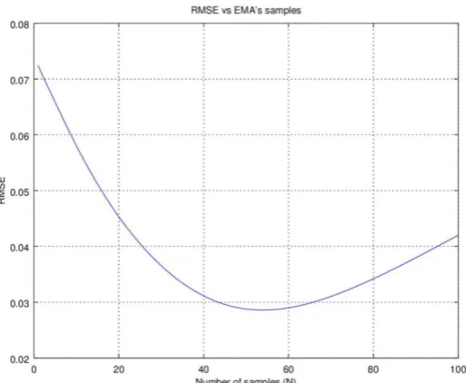
Figure 18. RMSE versus number of samples 𝑁

[image:29.595.170.427.70.281.2]

The lowest RMSE value obtained was about 0.03 m/s, for 𝑁 = 54 (𝛼 ≅ 0.036). Furthermore, the EMAd reference for this specific number of samples is shown in Figure 19 below. Note the encoder readings fairly fit, thus from now on in this section, reference will correspond to the EMAd reference and is considered as the ground truth speed for all RMSE calculations. It is relevant to notice, however, that this EMA is a post-processing technique, being implemented offline exclusively.

Figure 19. Exponential moving averaged reference for N=54, alongside the encoder readings

(30)

[image:30.595.146.450.74.325.2]

30

Figure 20. Accelerometer readings based on the test sequence

Moreover, it is relevant to notice the movement-end check impact on the estimated speed, which forces the output to zero only after twenty-five (25) consecutive zero readings, clearly visible when the reference is set to zero. Moreover, notice that estimation procedure does drift over time, which is evident for the first two iterations and the fifth, due the fact their longer duration, when this effect becomes more visible. Finally, it is clear the speed estimation is less accurate than the encoder readings, but outputs data three times faster (150 Hz) with the current data processing required by the speed estimation algorithm.

Complementary Filter

The IMU and encoder data are fused through a complementary filter, in order to reduce the overall noise of the derived speed before forwarding such information to the Pre-Kalman filter and, subsequently, to the Kalman filter itself, which is further explored in the next chapter. Both 1st_{and 2}nd

order complementary filters were implemented offline to simplify the procedure of tuning their respective gains. Additionally, considering the complementary filter implementation consists basically of hard-coding equations (2.4) for the 1st_{order or (2.7-2.11) for the 2}nd_{order, the bottleneck in terms}

of how fast the robotic system can provide a filtered output is not influenced by the additional operations. Thus, the offline implementation for tuning the gains should present the same behavior as the real one, given a 150Hz frequency is respected.

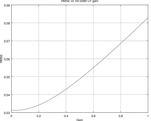
Initially, the 1st_{order complementary filter was tested by varying the gain}_{𝐾 from 0 to 1, which}

corresponds to not considering or only considering the accelerometer speed estimation, respectively.

For each gain, RMSE is computed based on the EMAd reference value and the filter’s output, which

(31)

[image:31.595.155.443.77.308.2]

31

Figure 21. RMSE versus 1st_{order CF gain}

The smallest and consequently the best RMSE obtained was 0.0312 m/s, which corresponds to a gain of 𝐾 = 0.02. Note that this value represents the filter outputs reliable speeds when the accelerometer speed estimation is given a 2% weight, meanwhile the encoder readings 98% weight. With the gain properly defined, the complementary filter was implemented and the whole test performed once more. The results were logged and plotted, as shown in Figure 22 below. Note both the reference and the encoder values are hardly visible, with the filter smoothly fusing the data and outputting a more stable speed.

Figure 22. 1st_{order complementary filter results}

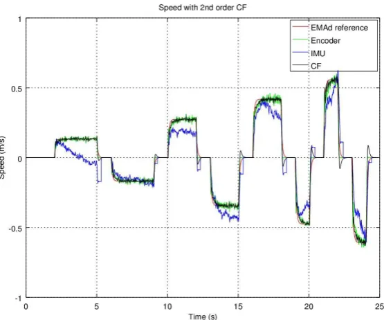
Although the 1st_{order filter presented fairly good results, the 2}nd_{order complementary filter was also}

[image:31.595.144.454.453.706.2]

(32)

32

more complex structure is worth to be chosen instead of the 1st_{order filter. The procedure applied to}

the 1st_{order filter is repeated, with the gain 𝐾 being varied from 0 to 20 and each respective RMSE}

[image:32.595.148.447.138.387.2]

calculated. The results are depicted in Figure 23 below:

Figure 23. RMSE versus 2nd order CF gain

Based on Figure 23 above, it is evident the 2nd_{order CF is rather unstable for this system in terms of}

RMSE. However, in order to fully check its behavior, the filter was implemented and tested with 𝐾 = 18, which corresponds to the best RMSE obtained (0.0322 m/s) – note that based on the RMSE, it is possible to conclude this implementation is worse than the 1st_{order one, that presented a smaller}

value: 0.0312m/s. The logged data was plotted and is shown in Figure 24 below. Note, however, that such implementation behaves properly and its output is similar to the 1st_{order, except when the speed}

(33)

[image:33.595.160.438.71.302.2]

33

Figure 24. 2nd_{order complementary filter results}

Comparison

In summary, both 1st_{and 2}nd_{order complementary filter implementations had similar performances,}

with the former slightly outperforming the latter. However, the 2nd_{order version requires extra}

memory, is slightly harder to implement, and presents an undesirable behavior (i.e. overshoot) which

may further influence the Kalman filter’s behavior. Due to these facts, the 1st_{order complementary}

filter was chosen to be used. Another interesting point is that although the RMSE of the 1st_order

version is higher than the pure encoder readings, the output of the filter itself has a smaller standard deviation (0.25699 in comparison to 0.24778), thus is more stable. Figure 25 compares both filter

versions’ implementations, for the whole test sequence.

[image:33.595.161.435.490.715.2]

(34)

34

Not only does the complementary filter reduce the overall standard deviation, but it also improves the sampling frequency of the speed. Previously, the speed could only be updated once every 20 milliseconds (50 Hz) due to the encoder limitation. By combining the encoder readings with the accelerometer speed estimation, one can poll at a much faster rate: every 6 milliseconds (166 Hz), about 3.3x faster. It is advisable, however, to retrieve data at a lower rate due the fact the system might be late when asynchronous events (i.e. references update) triggered by a master (i.e. tracking system) must be processed. In practice, the refresh rate used corresponds to 140 Hz.

Finally, the robotic system comprises the implementation of this technique due the fact it is considered the low-level control system. Hence, it is responsible for driving the motors, providing the current (filtered) speed, and additionally the gyroscope data required by the Pre-Kalman filter.

2.5 Communication protocol

Communication between the robotic system and a master (e.g. tracking system), more specifically the MegaPi board – PC (or ideally Zynq) data exchange must respect guidelines in order to proper send or receive data. Thus, a (micro)protocol under certain bus configurations was implemented, and will be addressed in this section. Such protocol is serial-based and implements data transfer with the Most Significant Byte being sent first (MSB first), and neither CRC nor ACK are implemented, to keep it as simple and fast as possible.

Data transfer is implemented through an UART bus, with both devices configured as follows: • Baud rate: 5000000 bps (62.5 kbps) – advisable to increase it in the future

• Word length: 8 bits • Stop bit(s): 1 • Parity: None • Flow control: None

The only and essential communication between the robotic and tracking systems is full-duplex, with both systems being able to send and receive data. Currently, two (2) message packets are supported, one for retrieving sensor data and another for setting new speed references. These packets are composed, generally, by a synchronization word (2 bytes), a command byte (1 byte), and data bytes. The former is used for synchronization purposes, the command is dedicated to specifying the requested functionality, followed by data bytes when applicable.

(35)

35

Figure 26. Master (tracking system) – Robotic system sensor data request (top) and response (bottom) data packets

Figure 27. Master (tracking system) – Robotic system references data packet

Requesting sensor data corresponds to sending three bytes, the sync word and the corresponding command (0x00). The robotic system replies with: current speed, yaw, pitch and roll (4 bytes each). A synchronization word is also added in the beginning of such message; thus, the total number of bytes sums up to 19 bytes for the response. Setting speed references requires 11 bytes in total to be sent: sync word, command (0x01), followed by the right and left reference speeds (4 bytes each). Note that all speed values are in RPM so data is platform-independent and a simple conversion is required to be done in another platform. Furthermore, positive and negative references correspond to moving forwards and backwards, respectively. Gyroscope data, on the other hand, is pre-processed (i.e. converted to °/s) due to the fact its sensitivity and other device-specific configurations should not be relevant to the master.

(36)

36

2.6 Final Implementation

[image:36.595.232.362.183.382.2]

With each component of the robotic system properly defined and tested, it is possible to merge them to compose the whole final implementation. This section presents an overview of the complete robotic system in terms of structure, hardware and software, with the setup itself being depicted in Figure 28 below.

Figure 28. Robotic system final setup

In addition to the components previously discussed, a camera is attached to the robotic system, as shown in Figure 28 above. Note, however, that such device is only placed together with this system, but it is part of the tracking system which will be discussed in the next chapter. Moreover, the current setup does not comprise a dedicated board (i.e. Zynq) that would perform the high-level operations related to the camera, due the fact the tracking system is running on a PC that connects to the robotic system with an USB cable. Ideally, the PC should be replaced by another board and the communication between systems realized with direct UART connections – Tx, Rx, VCC and GND.

2.6.1 Hardware

(37)

[image:37.595.135.465.77.278.2]

37

Figure 29. Final hardware architecture of the robotic system

Notice the IMU module was placed on the same platform as the battery (check Figure 28), which

defines the reference axis for the module’s data: the positive X axis points to the front, positive Y to the left and positive Z to the top of the robot, respectively. This configuration directly impacts the data signaling retrieved from the module, and was taken into consideration during development. Based on

the module’s orientation, heading (or yaw), pitch and roll are rotation around the XY, XZ and YZ planes, respectively, with the gyroscope and accelerometer data correspondence being summarized in Table 2 below.

Table 2. Movement type, axis, and signaling correspondence for the IMU module

2.6.2 Software

In terms of software, the robotic system is responsible for retrieving and processing IMU and

encoder’s data, alongside applying the complementary filter and driving the motors. Moreover, it

must comply to the µprotocol discussed and react to asynchronous serial events. It is relevant to notice that the software runs in a single-core microcontroller, in a sequential manner, with the Arduino IDE being the development tool used. The first step is initializing peripherals, as shown in Figure 30 below:

Figure 30. Robotic system’s initialization procedure

Initialization is rather simple, with relevant I/O pins begin initialized first, followed by the encoder

motors which requires setting up related timers for PWM and encoders’ interrupts. Then, the IMU Accelerometer Gyroscope Positive Negative

Heading - Z Turning left Turning right Pitch - Y Going downhill Going uphill

Roll - X Rolling right Rolling left Linear X - Going forward Going backward

Signal meaning

Movement Axis

Initialize pins Initialize

encoder motors Initialize IMU Initialize UART