J.A.Kreuzberg
September 4, 2016
Abstract
This paper does research for a local search heuristic approach to compute a revenue maximizing single item auction, called an optimal auction. We try to find the maximal expected revenue of the auctioneer by maximizing the expected payments of the bidders. We show that this problem can be reduced to finding an optimal order of the possible types of the bidders. We use that insight to propose a simple local search algorithm for computing an optimal auction.
1
Introduction
An auctioneer wants to sell one item to a group of bidders where each bidder has private infor-mation about their value for the item. There already is an analytical approach of Myerson that computes the maximal expected revenue of the auctioneer for auctions in this setting. In this pa-per we search for a different approach to compute the maximal expected revenue. This approach appears to be a local search heuristic that has potential to be applied in auction settings where the analytical approach of myerson doesn’t work anymore.
2
The optimal auction
2.1
The definition of an auction
To get a clear image how an auction is defined formally, there will first be introduced some basic notation, which will also help clarifying some of the model assumptions.
Assume an auctioneer wants to sell a single item tonbidders. Every bidder has a private valuation for this item, which is also known as a bidder’s type. A bidder has a certain type, which is unknown for the other bidders and the auctioneer. Since a bidder’s type is private information, the auction-eer doesn’t know what type each bidder has. The auctionauction-eer only knows that each bidder has a type spaceTj consisting of all possible types bidderj could have: Tj ={t1, . . . , tb}, wherej= 1, . . . , n
andtb is the maximum type a bidder can have for the item withb∈N. The assumption is made
that all bidders are identical so the type space of each bidder is the same. Furthermore a bidders type is drawn from his distribution independently from the other bidders. Since all thenbidders have their own type space, the type space of the auction looks likeTn=T1∪· · ·∪Tn={t1, . . . , tb}.
The type distribution vectorϕthat describes the probability to be a certain type from the type-spaceT, needs to satisfyP
ϕi = 1 and ϕi >0 for i= 1, . . . , b. So the input for an auction is a
stochastic type vector (t1, . . . , tn) that consists of the types each bidder has. This means that the
An auction always consists of two mappings: an allocation rule and a payment rule. The al-location rulea(t) is a function that will determine which bidder will get the object for any given type vectort. This is a mapping from the type space Tn ={1, . . . , b} to the space of allocations
A={0,1}:
(t1, . . . , tn) a
→(a1(t), . . . , an(t))
In a single item auction there can only be one good allocated among the bidders, soP
aj(t)≤1.
An example of an allocation rule could be that the item will go to the bidder with the highest type or randomly assigned among all bidders with the highest type. This allocation rule is also used in a vickrey auction with reserve price [4]. In this example there are three possible scenario’s for the allocation of the item.
a(t) =
(0, . . . ,1, . . . ,0) if one bidder has the highest type 0, . . . ,m1, . . . ,m1, . . . ,0
ifmbidders have the highest type
(0, . . . ,0) ifti< t∅ for alli= 1, . . . , n
As already said, the j-th index of the allocation vector corresponds to bidderj, wherej= 1, . . . , n. Since there is assumed that the bidder’s type distribution is i.i.d., one can say without loss of gen-erality that it is also possible to look at one bidder only. The allocation rule for a bidder, say bidderj, is:
aj(t) =
1 if bidder j has the highest type 1
m if bidderj andm−1 other bidders have the highest type
0 if there exists ati such thattj < ti (where i =∅is allowed)
Once the allocation rule has assigned a winner, the corresponding payment has to be made by this bidder. This payment follows from the payment rule. A payment rule also is a function that maps a type vectortto a vector of paymentsπ, whereπj(t)∈Rforj= 1, . . . , n:
(t1, . . . , tn) π
→(π1(t), . . . , πn(t))
An example of a payment rule is that the payment rule claims that the winning bidder has to pay an amount equal to his type. In that caseπ(t) looks like:
π(t) =
(
(0, . . . , tj, . . . ,0) if bidder j has the highest type
(0, . . . ,0) ti< t∅ for alli= 1, . . . , j, . . . , n
When the situation occurs thatmof thenbidders have the highest type, it doesn’t matter which bidder eventually wins the auction. This winning bidder has to pay the price of this highest type to the auctioneer. An auction with this allocation and payment rule is also known as a first price auction.
So now it is clear how an auction is defined. The input for an auction is a stochastic type vector
t, depending on the reported types of the bidders. Applying the allocation rule and payment rule gives as output the winning bidder and the corresponding payment :
(t1, . . . , tn) a
→(a1(t), . . . , an(t))
(t1, . . . , tn) π
→(π1(t), . . . , πn(t))
2.2
The expected allocation and payment
bidderj wins the auction with typeti∈ {t1, . . . , tb}. Due to the stochastic input, we have to take
the expectation over all possible types of other bidders and fix the type of bidder j. Therefore the type vector t−1 is defined as the types of all other bidders except the type of bidder j:
t−1= (t1, . . . , tj−1, tj+1, . . . , tn). Herefore the expected allocation can be expressed as follows:
pi=
X
t−1∈Tn−1
a(t−1|bidderj has typeti)·ϕ(t−1)
Here a(t−1|ti) is the allocation of the object with input t−1 and the type of bidderj fixed toti.
This allocation can only be made if the corresponding type vector t−1 occurs. This probability is given byϕ(t−1) . Note that it can occur that the type ti of bidder j is below the type of the
auctioneer,t∅. In that casepi= 0.
With this expected allocation, the probability that a bidder wins the auction can be described more in detail. Recalling the assumption that all bidders are independent and identical, every bidder has the same probability to win the auction. If there are n bidders who participate in the auction, the probability that bidderj would win the auction is lower or equal to n1 because we have to take into account that there is a probabillity that the item won’t be sold. Because it is unknown which type bidder j has, one must consider all possible types. This leads to the following:
P{bidder j wins the auction}
=
b
X
i=1
P{Bidder j wins the auction| Bidder j has typeti} ·P{Bidder j has typeti}
=
b
X
i=1
pi·ϕi≤
1
n
This expression is obtained by using the Law of Bayes to implement the condition that bidderj
has typeti.
The vector phas the following structure: p = (p1, . . . , pb). There also is a probability that the
type of a bidder is below the type of the auctioneer. The probability that the auctioneer won’t sell the item, so the expected allocation of the auctioneer, is denoted asp∅. This probability consists of all probabilities that a bidder with a type below the auctioneer’s type will win the auction:
p∅=
X
i:ti<t∅
pi
This makes sense because the auctioneer won’t sell the object if the highest type is below her type.
The expected payment can be derived from the payment rule. The amount a bidder with typeti
expects to pay, Πi, can be derived almost the same way as the expected allocation:
Πi=
X
t−1∈Tn−1
π(t−1|bidderj has typeti)·ϕ(t−1)
The expected payment of a bidder with type ti is the payment he should pay according to the
payment rule under the condition that this bidder has type ti and the types of the other bidders
are described byt−1. Again the corresponding type vectort−1has to occur.
2.3
Assumptions for the auction
tj , is denoted asν(pj|ti). The expression for the expected valuation is as follows:
ν(pj|ti) =ti·pj ∀i, j∈ {1, . . . , b}
The first assumption is that a bidder must obtain a non-negative surplus from participating in the auction. This means that the payment the auctioneer charges to a bidder is bounded by the expected valuation of a bidder.
Πi≤ν(pi|ti)∀i∈ {1, . . . , b}
When this assumption doesn’t hold, the auctioneer could charge infinite payments from the bid-ders.
The second assumption that must hold is that bidding truthful gives a higher surplus as bid-ding non-truthful. In this way bidders won’t report another type as their true type. It could be that a choosen allocation and payment rule gives the incentive to report different than your true type. In 1981, the american economist named Roger B. Myerson, proved that for every allocation and payment rule that form an auction, there is a corresponding auction where these two assump-tions hold. For this reason, without loss of generality, the assumption can be made that bidders are truthful in reporting their type when searching for the optimal auction. The incentive to bid your type truthfully is also known as the Lowercase Revelation Principle [3]:
ν(pi|ti)−Πi ≥ν(pj|ti)−Πj ∀ti, tj ∈T
3
Mathematical foundations for the optimal auction
In section 2 the auction is formally described. This was neccessary to obtain a good understanding of the assumptions for the model. Now we can focus on optimizing the expected revenue of the auctioneer under the assumed conditions. The expected revenue of the auctioneer is denoted as
E[R]. The expected revenue of the auctioneer constists of the the expected payments from all the
nbidders. Recalling the argument from section 2 that all bidders are identical and independent from each other, it is sufficient to focus on the expected payment of one bidder only. Since the auctioneer doesn’t know the type of a bidder, conditioning on the possible type is neccesary. So the expected payment of a bidder consists of the sum of the expected payments of a bidder with typeti under the probability that the bidder has typeti, fori= 1, . . . , b.
E[R] =
n
X
j=1 Πj =
n
X
j=1
b
X
i=1
Πij·ϕi=n· b
X
i=1 Πi·ϕi
To compute the expected payments, the assumption of truth telling will be rewritten. The lower-case revelation principle gives:
ν(pi|ti)−Πi ≥ν(pj|ti)−Πj ∀ti, tj ∈T
Now takej =i−1.
ν(pi|ti)−Πi≥ν(pi−1|ti)−Πi−1
⇐⇒Πi−Πi−1≤ν(pi|ti)−ν(pi−1|ti)
⇐⇒Πi−Πi−1≤ti(pi−pi−1)
Because the auction is seen from the perspective of the auctioneer, it is not difficult to understand that given some value for Πi−1, the auctioneer will charge Πi as large as possible. This yields
Because this holds for every typeti, one can construct a formula for every expected payment of
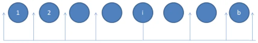
typeti that only depends on the probabilitiespi. In figure 1 this is illustrated in a directed type
graph. This graph consist of b vertices, where each vertex corresponds with a certain type. The weight of going fromti−1→tiisti(pi−pi−1)∀i= 1, . . . , b. For computing the expected payments
we add a dummy vertex to the type graph. Hereby it is possible to compute the maximal expected payment from typeti by finding a shortest path for 0→ti. Here Π0= 0 andν(p0|ti) = 0 because
the dummy vertex is not linked to a type.
0
ν(p1|t1)
t1
ν(p2|t2)−ν(p1|t2)
ν(p1|t1)−ν(p2|t1)
t2 ti
ν(pi+1|ti+1)−ν(pi|ti+1)
ti+1
ν(pi|ti)−ν(pi+1|ti)
tb
Figure 1: The directed type graph
In section 2 we stated the two assumptions that the surplus of a participating bidder is non-negative and that the bidders report their type truthfully. To make sure these assumptions still hold in the type graph, there may not exist cycles of negative length. Only when there are no cycles of negative length, the shortest path for 0→ticorresponds with the expected payment Πi.
Consider the cycle fromti→ti+1 and back.
[ν(pi+1|ti+1)−ν(pi|ti+1)] + [ν(pi|ti)−ν(pi+1|ti)]≥0
⇐⇒ti+1(pi+1−pi) +ti(pi−pi+1)≥0
⇐⇒(ti+1−ti)(pi+1−pi)≥0
⇐⇒pi+1−pi≥0
Here we used the monotonicity of the types to derive the last step.
Since this holds for every i∈ {1, . . . , b}, it follows that the expected allocationpis monotone in the types. This condition must hold while maximizing the expected revenue of the auctioneer.
In the directed type graph of figure 1 the edges from ti → tk, k > i+ 1 are not illustrated,
but they do exist. The shortest path for the expected payment Πiappears to be the directed path
from 0→ti. Using the triangle inequality we can show that a directed path in the type graph of
figure 1 is always shorter as skipping a vertex. To show this, take three random neigbour vertices,
ti−1, ti, ti+1, as is illustrated in figure 2.
ti−1
ν(pi|ti)−ν(pi−1|ti)
ti
ν(pi+1|ti+1)−ν(pi|ti+1)
ν(pi+1|ti+1)−ν(pi−1|ti+1)
ti+1
Figure 2: Triangle inequality
ti−1→ti+1and skip the vertex ti :
[ν(pi|ti)−ν(pi−1|ti)] + [ν(pi+1|ti+1)−ν(pi|ti+1)] =ti(pi−pi−1) +ti+1(pi+1−pi)
=ti+1pi+1+ (ti−ti+1)pi−tipi−1
≤ti+1pi+1+ (ti−ti+1)pi−1−tipi−1 =ti+1(pi+1−pi−1)
=ν(pi+1|ti+1)−ν(pi−1|ti+1)
In this proof we used the monotonicity of the types and the monotonicity of p such that (ti−
ti+1)pi≤(ti−ti+1)pi−1. So the maximal expected payment Πiis indeed the directed path 0→ti
among all the verticest1, . . . , ti−1. Therefore the maximal Πi can be expressed as follows:
Πi= i
X
s=1
ν(ps|ts)−ν(ps−1|ts)
=
i
X
s=1
tsps−tsps−1
=
i
X
s=1
ts(ps−ps−1)
=tipi− i−1
X
s=1
(ts+1−ts)ps
Recalling the formula to compute the expected revenue of the auctioneer:
E[R] =n·
b
X
i=1
ϕi·Πi
=n·
b
X
i=1
ϕi· tipi− i−1
X
s=1
(ts+1−ts)ps
!
=n·ϕ1t1p1+ϕ2(t2p2−(t2−t1)p1) +· · ·+ϕb[tbpb−(tb−tb−1)pb−1− · · · −(t2−t1)p1)]
=n·[t1ϕ1−(t2−t1)ϕ2− · · · −(t2−t1)ϕb]p1
+ [t2ϕ2−(t3−t2)ϕ3− · · · −(t3−t2)ϕb]p2+· · ·+ [tb−1ϕb−1−(tb−tb−1)ϕb]pb−1+ϕbpb
=n·
b
X
i=1
tiϕi−
"
(ti+1−ti) b
X
s=i+1
ϕs
#! pi
=n·
b
X
i=1
ti−
1−Φ(i)
ϕi
(ti−ti−1)
ϕipi
=n·
b
X
i=1
v(i)ϕipi
Here Φ(i) is the cumulative distribution function such that: Φ(i) =
i
P
s=1
ϕs. The function v(i) is
called the virtual valuation according to typeti:
v(i) =ti−
1−Φ(i)
ϕi
For simplicity assume that v(i) is monotone ini. This is an important assumption because now only distibutions ϕ are allowed such thatv(i) is monotone. When v(i) wouldn’t be monotone, bidders could get the incentive to report a lower type as their true type to obtain a higher virtual valuation. So to assume the bidders report their type truthfully,v(i) must be monotone [5].
The other partϕipican be seen as the probability that a bidder has typeti and wins the auction
with this type. This can be transformed to the probability that a typeti wins the auction, which
is defined asxi.
So the final expression for the expected revenue of the auctioneer is as follows:
E[R] =n·
b
X
i=1
v(i)ϕipi
=n·
b
X
i=1
v(i)xi
Since the goal is to find the maximum value forE[R], it is clear to see that the x’s with the highest
virtual valuation has to be chosen as high as possible. Recalling the assumption
b
P
i=1
xi≤ n1 , there
is a maximum of 1
n to be distributed over the vector (x1, . . . , xb).
One could think that thexiwith the highest virtual valuation equals 1n. However the composition
of vector x, actually the composition of the vector punder the probabilityϕ, has to be feasible. Feasibility means that the representation of the expected allocation can be mapped back to a real auction.
This feasibility can be obtained by using Border’s Theorem [1]. Border’s Theorem claims that the expected allocationpi is feasible ⇐⇒
n·X
i∈S
ϕipi≤1−(
X
i /∈S
ϕi)n ∀S⊆ {1,2, . . . , b}
The left hand side represents the expected distributed quantity of the good to the bidders with types in S. The right hand side represents the probability that one or more bidders have a type inS.
Rewriting this formula, we derive the following:
n·X
i∈S
ϕipi≤1−(
X
i /∈S
ϕi)n ∀S ⊆ {1,2, . . . , b}
⇐⇒ X
i∈S
ϕipi≤
1−(P
i /∈S
ϕi)n
n
⇐⇒ X
i∈S
xi≤
1−(P
i /∈S
ϕi)n
n
By definingG(S) = 1−(P
i /∈S
ϕi)n
n , the final condition for feasibility is:
X
i∈S
xi≤G(S)∀S⊆ {1,2, . . . , b}
Note that we want to maximize (x1, . . . , xb) so that the expected revenue will be maximal. We
know that the virtual valuations are montone in the types so we maximize (x1, . . . , xb) according
to their virtual valuation. Sincev(1)≤v(2) ≤ · · · ≤v(b), we maximize (x1, . . . , xb) in the same
following inequalities must hold:
xb≤G({b})
xb+xb−1≤G({b, b−1})
. . .
xb+xb−1+· · ·+x1≤G({b, b−1, . . . ,1})
In each condition we can isolatexi such that:
xb≤G({b})
xb−1≤G({b, b−1})−xb
. . .
x1≤G({b, b−1, . . . ,1})−xb−xb−1− · · · −x2
Here we can apply the algorithm of Jack Edmonds. With Edmonds’ Greedy algorithm we first maximize xb, after that xb−1, untill we reach x1. So the optimal feasible solution x can be
computed by replacing the inequalities through equalities.
xb=G({b})
xb−1=G({b, b−1})−xb=G({b, b−1})−G({b})
. . .
x1=G({b, b−1, . . . ,1})−xb−xb−1− · · · −x2
Now we know how to obtain the optimal solution (x1, . . . , xb) by this greedy algorithm, we need
to prove the feasibility of this greedy solution. We do this by using two equivalent properties of the functionG(S). It appears that the functionG(S) is a submodular set function which is non-decreasing and non-negative. Such a submodular set function G(S) has the following equivalent properties:
1. G(S∩R) +G(S∪R)≤G(S) +G(R)∀S, R⊆ {1, . . . , b}
2. G(S∪ {l})−G(S) is non-increasing in S∀S⊆ {1, . . . , b}, l /∈S
Due to the submodularity ofG(S), we can prove the feasibility of the solution (x1, . . . , xb).
To show: X
i∈S
xi ≤G(S)∀S⊆ {1,2, . . . , b}
The idea is to use induction to show this holds for every cardinality of the subsetS. So the first step is to verify this for|S|= 1. Choose an arbitraryj ∈ {1, . . . , b}, then
xj:=G({1,2, . . . , j})−G({1,2, . . . , j−1})≤G({j}) forS ={j}
Here the property of submodularity is used for computing xj such that R ={1, . . . , j−1} and
S={j} forj∈ {1. . . . , b}.
Now assume P
i∈S
Let (i1, . . . , ib) be an order of the type set{1, . . . , b} such thatik∈ {1, . . . , b}fork= 1, . . . , b
LetS ={i1, . . . , il+1}
=S0∪ {i1}, where typei1 is the minimum of this set.
Sincexi1 =G({i1} ∩S
0) +G({i
1} ∪S0)−G(S0) =G(S)−G(S0)
=⇒ X
i∈S
xi=
X
i∈S0
xi+xi1
≤G(S0) +xi1
≤G(S0) + [G(S)−G(S0)] =G(S)
Now we proved feasibility for the solution x, the maximization problem to obtain the highest expected revenue is reduced to:
max
x n· b
X
i=1
v(i)xi
s.t. X
i∈S
xi≤G(S)∀S⊆ {1, . . . , b}
pi≤pi+1 ∀i∈ {1, . . . , b}
It is also possible to formally prove optimality for the solution x. From the primal problem of maximizing the expected revenue, one can construct a dual problem. By complementary slackness it can be shown thatxis an optimal solution for both the primal and dual problem so indeed is an optimal solution [2].
4
Local Search
In the previous section we derived the optimal solution by first maximizing xb, thenxb−1, until
x1. This actually is an order of types in which the correspondingxwill be maximized.
By applying the Edmonds’ Greedy Algorithm, the strategy is to look for which typei1the virtual valuation v(i1) has the highest value and first maximize this xi1. After that xi2 , for which the
virtual valuationv(i2) has the second highest value, will be maximized. This keeps going untill the type with the lowest priorityib is reached such thatxib will be maximized. One can see that
there actually has to be found an optimal order (i1, . . . , ib) to optimize the x vector such that b
P
i=1
v(i)xi will be maximal. Since the virtual valuations are monotone in the types, the order of
of virtual valuations is the same order of possible types. Therefore the following theorem can be stated:
Theorem 1 Searching for the auctioneer’s revenue maximizing auction can be reduced to finding an optimal order of possible types (i1, . . . , ib).
It occurs that types have a negative virtual valuation. If this happens, the correspondingxvalues are set to zero. Those corresponding x and so the expected allocation p have no influence on the expected revenue anymore. Those probabilities belong to the probability that the auctioneer won’t sell the item. So we can rewrite the formula forp∅:
p∅=
X
i:v(i)<0
4.1
Finding the optimal order of types
The optimal order (i1, . . . , ib) can be found by a local search heuristic on the possible types.
Choose a random type and analyze at which priority in the order it gives the highest expected revenue for the auctioneer. Doing this for all possible types, eventually it will give the optimal order of types. The local search heuristic is illustrated in figure 3.
Figure 3: Finding the optimal order of types
Actually finding the optimal order of types comes down to finding the order of virtual valuations. Due to the monotonicity of the virtual valuations we know that the optimal order for auctions this paper looks at, is (b, b−1, . . . ,1).
5
Computational results
After achieving the result that it is possible to obtain the optimal auction by a local search heuristic theoratically, it is interesting to verify this by computational results. There are two main questions to investigate:
1. Does the local search heuristic give the same expected revenue as the analytical approach of Myerson?
2. What influence has the type distribution on the expected revenue?
Furthermore it is interesting how the exected revenue reacts when the amount of bidders increases.
5.1
Does the local search heuristic give the same expected revenue as
the analytical approach of Myerson?
The straight answer to the question is that the local search heuristic indeed gives the same ex-pected revenue as the analytical approach of Myerson. This can be seen by the following example:
Example 1 Assume the following inputn= 10, T ={1,2, . . . ,14} , ϕ∼unif orm(0,14)
Using this input, we can compute the virtual valuations:
v(T) =[-12.0000 -10.0000 -8.0000 -6.0000 -4.0000 -2.0000 -0.0000
2.0000 4.0000 6.0000 8.0000 10.0000 12.0000 14.0000]
We can compute each xi by computingG(S) =
1−(P
i /∈S
ϕi)10
10 for the corresponding S. Every type
that has a negative virtual valuation, doesn’t have a probability to win the auction. Recalling the probability that the auctioneer won’t sell the item isp∅= P
i:v(i)<0
pi
According to the virtual valuations, the optimal order of types is (14,13, . . . ,1) so the expected allocation punder the probability ϕis
Therefore the expected allocation can be computed:
(p1, p2, . . . , p14) = [0 0 0 0 0 0 0 0.0038 0.0117 0.0315 0.0771 0.1741 0.3676 0.7328]
Here p∅= 7
P
i=1
pi = 0.0014.
From the virtual valuation and the solution x, we can compute the expected revenue of the auc-tioneer. So when there are 10 participating bidders, each having a type space {1,2, . . . ,14} and the type distribution is uniform, the expected revenue of the auctioneer is :
E[R] = 10·
14
X
i=1
v(i)xi= 12.3367
Using the same input, the analytical approach of Myerson gives the same output as the greedy algorithm.
5.2
What influence has the type distribution on the expected revenue?
Recalling the assumption that the type distribution ensures montone virtual valuations. So not all type distributions are feasible. When the probability of reporting a type changes, the expected revenue will be influnced by that. In example 1 the type distributionϕis uniform.
Soϕ1=ϕ2=· · ·=ϕ14=141
The following example has an exponential type distribution. First we need to check if an exponen-tial distribution gives monotone virtual valuations. In this example it holds thatϕ1≤ϕ2≤ · · · ≤
ϕb, so the virtual valuationsv(i) =ti−1−Φ( i)
ϕi (ti−ti−1) will be monotone in the types. The part
1−Φ(i)
ϕi (ti−ti−1) will decrease if the types increases so the virtual valuationsv(i) won’t decrease
in the typesti.
Example 2 The input for the auction is n= 10, T ={1,2, . . . ,14},
(ϕ1, ϕ2, . . . , ϕ14) =(0.0000 0.0000 0.0000 0.0000 0.0001 0.0002 0.0006 0.0016 0.0043 0.0116
0.0315 0.0855 0.2325 0.6321)
Using this input, we can calculate the virtual valuations:
v(T) = 10000·(-6.9989 -2.5747 -0.9471 -0.3484 -0.1281 -0.0471 -0.0173
-0.0063 -0.0022 -0.0007 -0.0002 0.0000 0.0001 0.0001)
Here the optimal order of types is also (14,13, . . . ,1) so the expected allocation punder the prob-abilityϕis
(x1, x2, . . . , x14) =[0 0 0 0 0 0 0 0 0 0 0 0.0000 0.0000 0.1000]
Therefore the expected allocation can be computed:
(p1, p2, . . . , p14) = [0 0 0 0 0 0 0 0 0 0 0 0.0000 0.0000 0.1582]
Here p∅= 11
P
i=1
pi = 2.9731·10−13≈0.
So when there are 10 participating bidders, each having the type space {1,2, . . . ,14} and the type distribution is exponential, the expected revenue of the auctioneer is :
E[R] = 10·
14
X
i=1
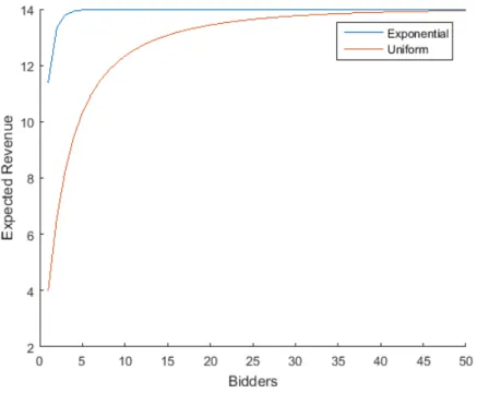
When we compare example 1 and 2, the results are very intuitive. The expected allocations of example 1 are more devided over the types. This makes sense because when a bidder has type 12 he still has a probability to win the auction since the probability that other bidders have a higher type is not that very high due to the uniform type distribution. Comparing this with example 2, we see that bidders with a type below 14 nearly have no probability to win the auction. This also makes sense because due to the exponential type distribution there is a very high probability that another bidder has type 14.
Furthermore we can see that the expected revenue is higher under an exponenital type distribution than a uniform type distribution. This also follows from the type distribution since in example 2 there is a high probability that a bidder has type 14.
It is also interesting to investigate what happens with the expected revenue if the amount of bidders increases. Figure 4 illustrates how the expected revenue is plotted against the amount of bidders.
6
Conclusion
The main conclusion of this paper is Theorem 1 that is stated in section 4. We are able to reduce the problem of computing the revenue maximizing auction to finding an optimal order of possible types.
We started by deriving a formula for the expected revenue that only depends on the expected payments of the bidders. It appeared that eventually the expected revenue only depends on the type distribution and the probability that a type wins the auction. So by finding an optimal order of possible types, those probabilities can be maximized according to the priority of the type. Among this way we were able to reduce the problem to finding an optimal order of possible types. Since the allowed type distributions ensures monotonicity in the virtual valuations, we already know what the optimal order of types is. But when it appears that the type distribution results in virtual valuations that are not monotone, the optimal order of types follows from the local search algorithm.
7
Future work
In this paper, we look at single item private value auctions. For these auctions we proved that under certain circumstances, the optimal auction can be derived from finding an optimal order of possible types. For these auctions we could also compute the expected revenue by the analytical approach of Myerson. But when the auctions consist of a more complex setting, it is almost never possible to compute the expected revenue by the analytical approach of Myerson. For this reason it is very interesting to investigate if this local search heuristic also gives the optimal auction if the auction consists of a more complex setting, like bidders with multi-dimensional types. To investigate this, the insight of this paper is very useful.
References
[1] Kim C Border. Reduced form auctions revisited. Economic Theory, 31(1):167–181, 2007.
[2] Bodo Manthey. Optimization modeling. pages 14–17.
[3] Roger B Myerson. Optimal auction design. Mathematics of operations research, 6(1):58–73, 1981.
[4] William Vickrey. Counterspeculation, auctions, and competitive sealed tenders. The Journal of finance, 16(1):8–37, 1961.