Inverse tone mapping

(1)

University of Warwick institutional repository:

http://go.warwick.ac.uk/wrap

A Thesis Submitted for the Degree of PhD at the University of Warwick

http://go.warwick.ac.uk/wrap/55447

This thesis is made available online and is protected by original copyright.

Please scroll down to view the document itself.

(2)

Inverse Tone Mapping

by

Francesco Banterle, BSc MSc

Submitted to the University of Warwick

for the degree of

Doctor of Philosophy in Engineering

The University of Warwick, School of Engineering

(3)

(4)

List of Figures

1.1 The HDR pipeline in all its stages. . . 2

1.2 A re-lighting example. . . 2

1.3 An example of capturing samples of a BRDF. . . 3

1.4 An example of HDR visualisation on a LDR monitor. . . 4

1.5 An example of a captured HDR image using Spheron HDR VR. . . 4

1.6 Synthetic objects re-lighting. . . 5

1.7 An example of quantisation errors during visualisation of LDR content on HDR monitors. . . 6

2.1 The elctromagnetic spectrum. . . 10

2.2 Light interactions. . . 11

2.3 The human eye. A modified image from Mather [129]. . . 13

2.4 The CIE XYZ colour space. . . 15

2.5 Ray tracing. . . 17

2.6 An example of state of the art rendering quality for ray tracing and rasterisation. 18 2.7 An example of HDR capturing of the Stanford Memorial Church. . . 20

2.8 The encoding of chrominance in Munkberg et al. [139]. . . 26

2.9 An example of the separation process of the LDR and HDR part in Wang et al. [206]. . . 30

2.10 An example of failure of the compression method of Wang et al. [206]. . . 31

2.11 Tone Mapping and real-world relationship. . . 32

2.12 An example of the applications of simple operators to Cathedral HDR image. . 36

(10)

2.14 An example of quantisation techniques. . . 39

2.15 An example of the operator proposed by Ferwerda et al. [63] of the Desk HDR image. . . 40

2.16 The various stage of Histogram adjustment by Ward et al. [107]. . . 41

2.17 The pipeline of the adaptation operator by Pattanaik et al. [156]. . . 42

2.18 A comparison between the method original method by Pattanaik et al. [156] and Irawan et al. [88]. . . 43

2.19 An example of the adaptive logarithmic mapping. . . 45

2.20 An example of the local TMO introduced by Chiu et al. [31]. . . 46

2.21 An example of the multi-scale observer model by Pattanaik et al. [155]. . . 48

2.22 An example of photographic tone reproduction operator by Reinhard et al. [169]. 49 2.23 A comparison between the TMO by Reinhard et al. [169] and the one by Ashikhmin [10]. . . 50

2.24 The pipeline of the fast bilateral filtering operator. . . 51

2.25 A comparison of tone mapping with and without using the framework proposed by Durand and Dorsey [194]. . . 52

2.26 A comparison between the fast bilateral filtering [194] and trilateral filtering [31]. 52 2.27 A comparison between the iCAM 2006 by Kuang et al. [101] and iCAM 2002 by Fairchild and Johnson [59]. . . 53

2.28 An example of tone mapping using the gradient domain operator by Fattal et al. [61]. . . 55

2.29 An example of Tumblin Rushmeier’s TMO [193]. . . 56

2.30 An example of the TMO by Krawczyk et al. [99]. . . 57

2.31 An example of the user based system by Lischinski et al. [118]. . . 59

2.32 An example of the automatic operator by Lischinski et al. [118]. . . 59

2.33 An example of the fusion operator by Mertens et al. [131]. . . 61

2.34 The HDR viewer by Ward [211] and Ledda et al. [110]. . . 62

2.35 The processing pipeline to generate two images for the HDR viewer by Ward [211] and Ledda et al. [110]. . . 63

(11)

2.37 The HDR Monitor based on LCD and LED technologies. . . 65

2.38 An example of the setup for the evaluation of TMOs using an HDR monitor as reference. . . 66

2.39 The Cornsweet-Craik-O’brien illusion used in Aky¨uz and Reinhard’s study [9]. 72 2.40 The Computer Science environment map encoded using the projection mappings. 74 2.41 The basic Blinn and Newell [21] method for IBL. . . 74

2.42 The basic Blinn and Newell [21] method for IBL. Explanation. . . 75

2.43 The Computer Science environment map filtered for simulating diffuse reflec-tions. . . 75

2.44 An example of classic IBL using environment maps. . . 76

2.45 An example of IBL evaluating visibility. . . 77

2.46 An example of evaluation of Equation 2.81 using MCS [170]. . . 78

2.47 A comparison between Monte-Carlo integration methods for IBL. . . 79

2.48 An example of stereo IBL by Corsini et al. [36] using the Michelangelo’s David model. . . 80

2.49 An example of dense sampling methods by Jonas et al. [197, 196] a toy cars scene. . . 80

3.1 An example of the need of working in the linear space. . . 83

3.2 A coloured edge region. . . 85

3.3 A grey-scale edge region. . . 86

3.4 The pipeline for bit depth extension using amplitude dithering in Daly and Feng’s method [41]. . . 88

3.5 The pipeline for bit depth extension using de-contouring in Daly and Feng’s method [42]. . . 89

3.6 An example of re-lighting of the Stanford’s Happy Buddha [73] using Landis’ method [105]. . . 89

3.7 The pipeline for calculating the maximum diffuse luminance value ω in an image in Meylan et al.’s method [133]. . . 90

3.8 The pipeline for the range expansion in Meylan et al. [133]. . . 91

(12)

3.10 The pipeline of Rempel et al.’s method [171]. . . 94

3.11 Application of Rempel et al.’s method [171]. . . 95

3.12 The pipeline of the system proposed by Didyk et al. [48]. . . 97

3.13 The interface used for adjusting classification results of the system proposed by Didyk et al. [48]. . . 98

3.14 The encoding pipeline for JPEG-HDR by Ward and Simmons [213, 214]. . . 100

3.15 The decoding pipeline for JPEG-HDR by Ward and Simmons [213, 214]. . . 102

3.16 An example of tone mapping using the multi-scale decomposition. . . 104

3.17 A comparison of tone mapping results for the Stanford Memorial Church HDR image. . . 105

3.18 The optimisation companding pipeline of Li et al. [115]. . . 106

3.19 The encoding pipeline for Backward Compatible HDR-MPEG by Mantiuk et al. [125]. 107 3.20 The decoding pipeline for Backward Compatible HDR-MPEG by Mantiuk et al. [125]. 109 3.21 The pipeline for range compression (red) and range expansion (green) proposed by Van Hateren [75]. . . 110

3.22 An example of Van Hareten’s algorithm with a frame of the RNL sequence. . . 111

3.23 The encoding pipeline presented of Okuda and Adam’s method [146]. . . 112

3.24 The decoding pipeline presented of Okuda and Adami’s method [146]. . . 113

4.1 The diagram of the used methodology. . . 116

4.2 An example of the iterations . . . 117

5.1 The pipeline of the framework for the iTMO for still images. . . 120

5.2 iTMO curves. . . 122

5.3 An example of saturation recovery using Equation 5.11 applied to the Cloud LDR image. . . 124

5.4 An example of expansion for well-exposed content for the Vineyard LDR image.125 5.5 An example of expansion for over-exposed content for the Venice Bay LDR image. . . 126

5.6 The pipeline for the generation of the expand map for still images. . . 127

(13)

5.8 An example of density estimation in 1D with different kernels with samples atx. 128 5.9 An example of 2D density estimation applied to an LDR version of the Bristol

Bridge HDR image. . . 128

5.10 An example of reconstruction and noise reduction using the expand map. . . . 129

5.11 An example of generated samples using MCS from Memorial Church HDR image. . . 130

5.12 An example of MCS applied to Pisa HDR image for generating 32 lights. . . . 131

5.13 An example of coloured expand map in the Redentore LDR image. . . 133

5.14 The pipeline of the framework for the iTMO for videos. . . 135

5.15 An example of filteringLd, Maxfor two scenes. . . 136

5.16 The pipeline for the generation of temporal expand maps. . . 137

5.17 An example of temporal density estimation applied to a 1D video sequence. . . 138

5.18 A comparison between automatic and non automatic density estimation for the 20-th frame of the sky sequence. . . 139

5.19 An example of automatic parameters estimation . . . 140

5.20 A comparison between methods for generating the expand map. . . 141

5.21 An example of expand map calculated at low resolution. . . 142

5.22 The computation flow showing the cooperation between CPU and GPU threads for the iTMO. The first thread in the top . . . 144

5.23 An example of density estimation on GPU using Cone and Gaussian kernel applied to Bristol Bridge LDR image. . . 145

5.24 An example of flattened 3D texture for storing a Gaussian temporal kernel usingrt=5. . . 146

5.25 The scheme of Joint Bilatereal Up-Sampling on the GPU. . . 148

5.26 An example of precomputed clamping. . . 149

6.1 The setup of experiments. . . 155

6.2 Linearisation of the luminance signal in the Dolby DR37P HDR Monitor. . . . 162

6.3 The eight images used for Experiment 1. . . 163

6.4 Environment maps used for the Experiment 2. . . 168

(14)

6.6 An example of the concentration HDR-VDP error in Scene 6 for the visualisa-tion task usingW. . . 176 6.7 This graph shows for the tested iTMOs that average HDR-VDP error (P(X)≥0.95)

increases moving from a diffuse material to a mirror one.. . . 178 6.8 Flickering evaluation forfireball.avisequence from Fedkiw’s website [62]. 179 6.9 Flickering evaluation forfireball-smoke.avisequence from Fedkiw’s

web-site [62]. . . 179 6.10 Flickering evaluation for sequence 1 frombbc-hd.movfrom BBC HD Gallery

[19]. . . 180 6.11 Flickering evaluation for sequence 2 frombbc-hd.movfrom BBC HD Gallery

[19]. . . 181

7.1 The pipeline for encoding HDR textures. . . 183 7.2 The pipeline for the decoding of a HDR Texture. . . 184 7.3 An example of failure of the use of a luminance separated colour space in S3TC

[image:14.595.124.530.49.719.2]

applied to Bottles HDR image. . . 187 7.4 An example of allocation varyingαfor the Eucalyptus’s grove HDR image. . . 189 7.5 An example of wrong parameters selection: a) The tone mapped image 15 from

Figure 7.11 with a region of interest in green. . . 190 7.6 An example of RGBE bilinear filtering for Image 17 from Figure 7.11. . . 192 7.7 An example of bilinear up-sampling using the proposed method for Image 11

from Figure 7.11. . . 192 7.8 The frequency of blocks interval in the log₁₀domain. . . 194 7.9 The calculation ofεRfor each block in the data set and each interval. . . 194

(15)

7.11 The 22 HDR textures used in the compression experiments. . . 196

7.12 The results of the comparisons using RMSE in the logarithm domain with the set in Figure 7.11 for RMSE. . . 198

7.13 The results of the comparisons using mPSNR with the set in Figure 7.11 for mPSNR. . 198

7.14 The results of the comparisons using VDP with the set in Figure 7.11 for HDR-VDP withP(X) =0.95. . . 199

7.15 A simple real-time application showing the Happy Buddha from the Stanford model repository with emphasis on texturing operations for timing. . . 201

7.16 The cache test on a GeForceGO 7300. . . 202

7.17 A close-up of the central window in Image 12 in Figure 7.11. . . 203

8.1 An example of the limits of the proposed algorithm. . . 206

A.1 An example of bilateral filter. . . 210

A.2 An example of joint bilateral up-sampling for rendering. . . 210

A.3 A comparison between bilateral and trilateral filter. . . 211

B.1 An example of typical artifacts of S3TC for the Clouds image. . . 213

C.1 This graph shows the increasing computational power in GFlops of GPUs by NVIDIA and CPUs by Intel from January 2003 . . . 215

C.2 The GPU Pipeline . . . 216

J.1 Scene 1. . . 234

J.2 Scene 2. . . 235

J.3 Scene 3. . . 235

J.4 Scene 4. . . 235

J.5 Scene 5. . . 236

J.6 Scene 6. . . 236

J.7 Scene 7. . . 236

J.8 Scene 8. . . 237

(16)

K.2 Images used in Experiment 2 using the Scene 1 environment map at exposure 0 for the glossy material. . . 239 K.3 Images used in Experiment 2 using the Scene 1 environment map at exposure

0 for the pure specular mateiral. . . 240 K.4 Images used in Experiment 2 using the Scene 2 environment map at exposure

0 for the diffuse material. . . 240 K.5 Images used in Experiment 2 using the Scene 2 environment map at exposure

0 for the glossy material. . . 241 K.6 Images used in Experiment 2 using the Scene 2 environment map at exposure

(17)

K.17 Images used in Experiment 2 using the Scene 6 environment map at exposure 0 for the glossy material. . . 247 K.18 Images used in Experiment 2 using the Scene 6 environment map at exposure

(18)

List of Tables

2.1 The main symbols used for the luminance channel.. . . 16

2.2 The table shows bits allocation for a 4×4 block in Munkberg et al.’s method [139]. . . 26

2.3 The table shows bits allocation for a 4_×4 block in Roimela et al.’s method [174]. . . . 28

2.4 The taxonomy of TMOs. . . 34

2.5 A summary of the built HDR devices and their main features. . . 61

5.1 The results of the performances of the CPU and GPU algorithm for static im-ages, and video for High Definition televisions resolutions. . . 151

6.1 An example of theai jpreference matrix for a subject and an image for the comparisons of iTMOs. . . 155

6.2 The dynamic ranges of the HDR images used in the first experiment Figure 6.3. . . 163

6.3 The results for Experiment 1 Overall Similarity. . . 165

6.4 The results for Experiment 1 Dark Areas. . . 166

6.5 The results for Experiment 1 Bright Areas. . . 167

6.6 The dynamic ranges of the HDR images used in the second experiment. . . 168

6.7 The results for Experiment 2 Diffuse Material. . . 170

6.8 The results for Experiment 2 Glossy Material. . . 170

6.9 The results for Experiment 2 Mirror Material. . . 171

6.10 The results of HDR-VDP comparisons for the Visualisation experiment. . . 174

6.11 The results of HDR-VDP comparisons for IBL tasks for the Diffuse Material. . 175

6.12 The results of HDR-VDP comparisons for IBL task for the Glossy Material. . . 175

(19)

7.1 Metrics comparisons. . . 200

B.1 The table shows the bit allocation for a 4_×4 block in S3TC Mode 1. . . 213

D.1 Preference tables for each Scene used for the Overall experiment.. . . 220

D.2 Consistency tables used for the Overall Experiment 1. . . 221

E.1 Preference tables for each Scene used for the Bright Areas experiment. . . 223

E.2 Consistency tables used for the Bright Areas Experiment 1.. . . 224

F.1 Preference tables for each Scene used for the Dark Areas experiment.. . . 226

F.2 Consistency tables used for the Dark Areas Experiment 1. . . 227

G.1 Preference tables for each Scene used for the Diffuse Material experiment. . . 228

G.2 Consistency tables used for the Diffuse Material Experiment 2. . . 229

H.1 Preference tables for each Scene used for the Glossy Material experiment. . . 230

H.2 Consistency tables used for the Glossy Material Experiment 2. . . 231

I.1 Preference tables for each Scene used for the Mirror Material experiment.. . . 232

(20)

Acknowledgement

Firstly, I would like to thank my supervisor Professor Alan Chalmers for giving me the oppor-tunity for doing a PhD. Alan helped me with precious advices and his encouragement everyday, he was always calm and positive. Even during the bad days, he firstly used to say me ”Don’t panic!”.

I must thank Dr. Patrick Ledda, a friend, that I met in Siggraph 2005, for proposing me as PhD student at Alan’s Laboratory. His advices and help during my PhD were very important for the development of my research on High Dynamic Range Imaging. Another special thank goes to Dr. Prof. Kurt Debattista, a friend, who always gave me good advices, help, and a lift back home. He helped me during my research with fruitful discussions and advices. More important, without him I couldn’t watch the Football World Cup 2006! Last but not least I thank Dr. Alessandro Artusi, a friend, that helped during my research. Both Patrick, Kurt, and Alessandro acted as unofcially secondary advisors during my PhD. Thanks guys for your terrific help!

I have made many friends in Bristol and Warwick over the last past years. I thank: Matt, Gavin, Yusef, Cathy, Veronica, Roger, Anna, Timo, Alexa, Marina, Piotr (ye will), Usama, Tom (Tom), Vibhor (a man of peace), Vedad (Jim), Belma, Jasminka, Jassim, Carlo, Elena, Alena, Remi, Silvester, Gabriela, Keith, Elemedin, and Mike. I had a great time in Warwick, especially at the pubs and other social events held in the Warwickshire. I greatly thank to Alan, Kurt, Alessandro, Paolo, Carlo (hello mate), Gabriela, Elisa, Patrick, Andrea, Keith, and Jassim for reading my thesis and giving me insightful comments and corrections. Thanks mates!! A special thank goes to the late Usama Mansour, a great man, a contributor of Warwick Visu-alisation Group, and more important a friend, that tragically died in a friendly football match in October 2007. All the best for his family.

I also thank my friends in Italy for discussions and great moments during my vacations in Italy: Francesco ”Paggio” Pasetto, Alberto ”Bubi” Rodoz, Laura ”Lalla”, Federico Tai, Mauro ”Hawk” Gambini, Sara Migliorini, Roberto Montagna, Matteo ”Caste” Castellarin, and Sebas-tiano Ridolfi. Moreover, I am grateful to my former supervisors in Italy at Computer Science department at University of Verona, Professor Andrea Fusiello and Professor Roberto Gia-cobazzi for their help and advices. A special thank to Professor Enrico Gregorio for his help on LA_TEX.

Throughout all PhD I had a great help from my family which supported me. This thesis would have never been possible without them. I greatly thank my family, my mother Maria Luisa and my father Renzo, and my brothers Paolo and Piero and his wife Irina. I also thank Elisa, ”ma ufi”, for discussing about Pearls, music, pizza, and Bar Aruuugola.

(21)

Declaration

The work in this thesis is original and no portion of the work referred to here has been submitted in support of an application for another degree or qualication of this or any other university or institution of learning.

Part of the work presented in this thesis was previously published by the author in the following papers:

• F. Banterle, P. Ledda, K. Debattista, and A. Chalmers.Inverse tone mapping. In GRAPHITE 06: Proceedings of the 4th international conference on Computer graphics and interac-tive techniques in Australasia and Southeast Asia, pages 349356, New York, NY, USA, 2006. ACM.

• F. Banterle, P. Ledda, K. Debattista, A. Chalmers, and M. Bloj.A framework for inverse tone mapping. The Visual Computer, 23(7):467478, 2007.

• F. Banterle, P. Ledda, K. Debattista, and A. Chalmers. Expanding low dynamic range videos for high dynamic range applications. In SCCG 08: Proceedings of the 4th Spring Conference on Computer Graphics, pages 349356, New York, NY, USA, 2008. ACM. • F. Banterle, K. Debattista, P. Ledda, and A. Chalmers. A gpu-friendly method for high

dynamic range texture compression using inverse tone mapping. In GI 08: Proceed-ings of graphics interface 2008, pages 4148, Toronto, Ontario, Canada, 2008. Canadian Informa- tion Processing Society.

• F. Banterle, P. Ledda, K. Debattista, A. Artusi, M. Bloj, and A. Chalmers.A psychophys-ical evaluation of inverse tone mapping techniques. To Appear in Computer Graphics Forum, 2009.

In all these publications the author had the role of leader, proposing and developing the main concepts and ideas.

Signed: Date:

(22)

Abstract

The introduction of High Dynamic Range Imaging in computer graphics has produced a nov-elty in Imaging that can be compared to the introduction of colour photography or even more. Light can now be captured, stored, processed, and finally visualised without losing information. Moreover, new applications that can exploit physical values of the light have been introduced such as re-lighting of synthetic/real objects, or enhanced visualisation of scenes. However, these new processing and visualisation techniques cannot be applied to movies and pictures that have been produced by photography and cinematography in more than one hundred years.

(23)

Chapter 1

Introduction

In the last two decades the introduction of High Dynamic Range (HDR) imaging by the com-puter graphics community has revolutionised the field and other areas such as photography, virtual reality, visual effects, and the video-games industry. Light can now be captured and fully utilised for various applications without the need to linearise the signal and to deal with clamped values. The very dark and bright areas of a scene can be recorded at the same time onto an image or a video, avoiding under-exposed and over-exposed areas. Traditional imaging methods do not use physical values and typically are constrained by limitations in technology that could only handle 8-bit per colour channel per pixel. Such imagery (8-bit or less per colour channel) is known as Low Dynamic Range (LDR) imagery.

(24)

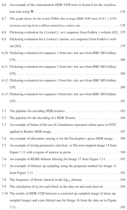
Figure 1.1: The HDR pipeline in all its stages. Multiple exposure images are captured and combined obtaining an HDR image. Then this image is quantised, compressed, and stored on the hard disk. Further processing can be applied to the image. For example, areas of high luminance can be extracted and used to re-light a synthetic object. Finally, the HDR image or processed ones can be visualised using traditional LDR display technologies or native HDR monitors.

HDR images/videos occupy four times the amount of memory of uncompressed LDR content. This is because light values are stored using three floating point numbers. This has a huge effect not only on storing and transmitting HDR data, but also in terms of processing performances. Efficient representations of floating point numbers have been designed for HDR imaging, and many classic compression algorithms such as JPEG and MPEG have been extended to handle HDR images and videos.

Lux

[image:24.595.114.524.54.257.2]

5.8e−01 1.5e+00 2.9e+00 5.2e+00 8.8e+00

(25)

Once HDR content is efficiently captured and stored, it can be utilised for various applications. A very popular application is the re-lighting of synthetic or real objects using HDR images, hence HDR data stores detailed lighting information of an environment. This information can be exploited for detecting light sources and using them for re-lighting objects, see Figure 1.2. Re-lighting is a very important application in many fields such as augmented reality, visual effects, and computer graphics. This is because the appearance of the image is transferred onto the re-lighted objects.

(a) (b)

Figure 1.3: An example of capturing samples of a BRDF: a) A tone mapped HDR image showing a sample of the BRDF from a Parthenon’s block [188]. b) The reconstructed materials in a) from many samples. Images are curtsey of Paul Debevec [188].

Another important application is to capture samples of the Bi-directional Reflectance Distribu-tion FuncDistribu-tion (BRDF) which describes how light interacts with a certain material. Then, these samples are used to reconstruct the BRDF, so HDR data needs to be captured for an accurate reconstruction, see Figure 1.3. Moreover, all fields which use LDR imaging can benefit from HDR imaging. For example, disparity calculations in computer vision can be improved in challenging scenes with bright light sources. This is because information in the light sources is not clamped, therefore disparity can be computed for light sources and reflective objects with higher precision than with clamped values.

(26)

these monitors reduces the complexity of further processing of the images/videos.

Lux

[image:26.595.114.525.442.650.2]

−1.0e+00 −1.0e+00 −1.0e+00 −1.0e+00 −1.0e+00

Figure 1.4: An example of HDR visualisation on a LDR monitor: on the left side an HDR image in false colour. In the centre two slices of the information: in the top an over-exposed image showing details in the dark areas, and in the bottom an under-exposed image showing details in the bright areas. On the right side the image on the left side has been processed to visualise details in bright and dark areas. This processing is called tone mapping.

1.1 The Need for LDR Content in HDR Applications

The weakest stage in the HDR pipeline is the capturing. At time of writing HDR video-cameras are still an open problem; a robust, noise-free, and high resolution HDR video-camera does not exist. However, there are two main solutions for taking HDR still images. The first one is to use automatic cameras such as the Spheron HDR VR [182], which currently costs around£45,000.

(27)

Moreover, with a bulky system and a setup of 10 minutes, it takes on average 8 minutes to capture a scene at 12 Megapixels, see Figure 1.5. The second solution is to use a normal camera. In this case, multiple-exposure images must be taken and then combined into an HDR image, as proposed by Debevec and Malik [47]. This is a long and manual process. A couple of minutes are needed for 6-8 exposures, plus a few minutes for combining the images into an HDR image. Moreover, the camera has to be still during all exposures, therefore a tripod is needed to avoid mis-alignments. However, both these two capturing methods have one common problem: time. Time is essential when capturing a picture, because a scene in the real world is for most of the time dynamic. For example, clouds can obscure the sun in a few seconds, or a car or a person can pass in front of the camera. Moreover, time is a very limited resource in some working fields. For instance, in visual effects the allocated time for capturing data on a cinematographic set is very small and a fast recording method can make a huge difference during post-production.

(a) (b)

Figure 1.6: Synthetic objects re-lighting: a) Stanford’s Lucy model [73] is re-lighted using an HDR image of St. Peter’s Cathedral. b) The same model is re-lighted using an LDR version of the image. Note that colours and hard shadows are lost. The original HDR image is courtesy of Paul Debevec [44].

(28)

[image:28.595.114.526.187.526.2]

photographs captured in more than one hundred years of photography and cinematography, cannot benefit from HDR applications. For example, an LDR panorama of a place that no longer exists cannot be displayed on HDR monitors or used as source for lighting. Re-lighting and visualisation are important tools for exploring the past and cultural heritage [122, 77]. Moreover, the introduction in the near future of HDR televisions would limit the access of LDR media to consumers.

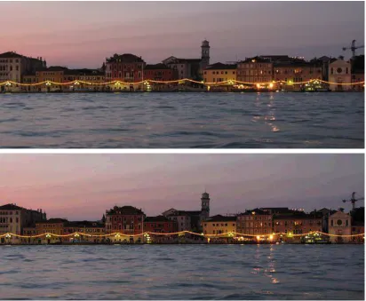
Figure 1.7:An example of quantisation errors during visualisation of LDR content on HDR monitors: On the top a LDR image of Venice bay. On the bottom a simulation of the same image on an HDR monitor. Linear stretching produces artefacts in the form of contouring.

In summary, while capturing HDR images and videos has not yet reached full maturity, LDR imaging has. LDR content at high resolution (more than 10 Megapixels) and at high speed (more than 100 frames per second) can be captured using devices that are cheap and available to consumers. However, LDR content fails to produce good results in HDR applications.

(29)

is achieved by proposing a series of algorithms that expands the dynamic range in LDR images and videos into HDR content on the fly at real-time frame rates. This expansion is followed by a reconstruction part, that generates plausible missing content and reduces quantisation arte-facts whenever possible. Furthermore, the approach is validated using psychophysical studies and image metrics. Finally, an application of expansion methods to tone mapped images is exploited to achieve an efficient compression algorithm.

1.2 Contributions

The major contributions of this thesis are:

• An in depth literature review on the field of HDR imaging. All parts of the HDR pipeline are taken into account: image/video capturing, storing, processing, visualisation, re-lighting, and validation.

• A review of the recent techniques for expanding LDR images/videos. Note that most of these techniques were developed after the publication of the core work presented in this thesis.

• The introduction and formalisation of the inverse tone mapping problem in the computer graphics field. How to generate HDR content from LDR images and videos is the dual of the tone mapping problem.

• A general framework for the expansion of LDR content into HDR that solves the inverse tone mapping problem. This framework can be applied to still images and videos and be accelerated using graphics hardware achieving real-time performances.

• The first study for the evaluation of performances of expansion methods using psy-chophysical experiments and computational metrics.

(30)

1.3 Thesis Structure

The thesis is structured in seven chapters as follows:

• Chapter 2: Backgroundintroduces an overview of the High Dynamic Range Imaging pipeline: how to create, store, process, and visualise HDR images and videos. More-over, a brief introduction on light quantities, human visual system, and colour spaces is provided.

• Chapter 3: Inverse Tone Mapping Operatorsis an in depth state of art on expansion methods for legacy content and compression schemes.

• Chapter 4: Methodologyintroduces the methodology which was used for the develop-ing of the new algorithm for expanddevelop-ing LDR content into HDR content.

• Chapter 5: An Inverse Tone Mapping Operatordescribes the framework of the the-sis, proposing a version for still images, videos, and an optimised implementation that exploits the power of modern graphics hardware.

• Chapter 6: Validation of Inverse Tone Mapping Operatorspresents two studies for the evaluation of performances of iTMOs. The first one is a pyschophysical study that employed paired comparisons. The second study is based on a perceptual metric.

• Chapter 7: Inverse Tone Mapping Application: HDR Content Compression is an application of inverse tone mapping to compress still images. While encoding is re-alised through tone mapping, decoding is achieved using inverse tone mapping. Further compression is achieved using a standard compression scheme, which is applied to tone mapped images.

(31)

Chapter 2

High Dynamic Range Imaging

HDR imaging is a revolution in the field of imaging, because it has introduced the use of physical-real values of light. This chapter introduces how to capture, encode, visualise and use HDR content. The chapter is structured into six sections:

• Section 2.1.1. Light, Human Vision, and Colour Space: This section introduces basic concepts of light, human vision, and colour spaces.

• Section 2.2. The Generation of HDR Images and Videos: This section describes the main techniques for generating HDR images and videos.

• Section 2.3. Encoding HDR Images and Videos: HDR content needs more memory to be stored than LDR content, because more information is needed to represent the full range of real world lighting. This raises the problem of efficiently storing images and videos. This section introduces the main encoding and compression schemes for HDR images and videos.

• Section 2.4.Tone Mapping: HDR content exceeds the dynamic range of current display technology such as CRT and LCD. Therefore, the visualisation of HDR images and videos on classic CRT and LCD displays is achieved by compressing intensities in the amplitude of the signal. This process is called tone mapping.

(32)

viewer and HDR displays. This section introduces these technologies that have been proposed in the last few years.

• Section 2.6.Evaluation of Tone Mapping Techniques: The large number of tone map-ping techniques introduced the need to determine which operator performs better than others for certain tasks, scenarios, and situations. This section introduces evaluation studies that have been proposed to measure the performances of tone mapping algo-rithms.

• Section 2.7. Image Based Lighting: One of the main applications of HDR content is image based lighting (IBL), which allows the realistic re-lighting of virtual and real objects. An overview on IBL is presented with emphasis on how to solve it.

2.1 Light, Human Vision, and Colour Spaces

This section introduces basic concepts of visible light and units for measuring it, the human visual system (HVS) focusing on the eye, and colour spaces. These concepts are very important in HDR imaging as it deals with physical-real values of light, from very dark values (i.e. 10−3 cd/m2) to very bright ones (i.e. 106 cd/m2). Moreover, the perception of a scene by the HVS depends greatly on the lighting conditions.

Figure 2.1: The elctromagnetic spectrum. The visible light has a very limited spectrum between 400 nm and 700 nm.

2.1.1 Light

(33)

travels in the space interacting with materials where it can be absorbed, refracted, reflected, and transmitted, see Figure 2.2. While the light is travelling, it can reach human eyes, stimulating them and producing visual sensations depending on the wavelength, see Figure 2.1.

Radiometry and Photometry define how to measure light and its units over time, space or angle. While the former measures physical units, the latter takes into account the human eye, where spectral values are weighted by the spectral response of the eye (y curve, see Figure 2.4). Radiometry and Photometry units were standardised by the Commission Internationale de l’Eclairage (CIE) [34]. The main radiometric units are:

• Radiant Energy(Ωe): is the basic unit for light, it is measured in joules (J).

• Radiant Power(Pe=Ω_dte): is the amount of energy that flows per unit of time (Js−1=W).

• Radiant Intensity (Ie = dP_d_ωe): is the amount of Radiant Power per unit of direction

(Wsr−1).

• Irradiance(Ee=_dAdPe_e): is the amount of Radiant Power per unit of area from all direction

of the hemisphere at a point (Wm−2).

• Radiance(Le= d

2_P

e

dAecosθdω): is the amount of Radiant Power arriving/leaving at a point

in a particular direction (Wm−2sr−1).

a)

b)

Figure 2.2:On the left side the three main light interactions: transmission, absorption, and reflection. In transmission, light travels through the material changing its direction according to the physical properties of the medium. In absorption, the light is taken up by the material that was hit and it is converted into thermal energy. In reflections, light bounces from the material in a different direction due the material’s properties. There are two main kind of reflections: specular and diffuse. On the right side: a) Specular reflections; a ray is reflected in a particular direction. b) Diffuse reflections; a ray is reflected in a random direction.

(34)

• Luminous Power(Pv): is the weighted Radiant Power, it is measured in lumens (lm) a

derived unit from candela (lm= cd sr).

• Luminous Energy(Qv): is the analogous of the Radiant Energy (lm s).

• Luminous Intensity(Iv): is the Luminous Power per direction, it is measured in candela

(cd or lm sr−1_).

• Illuminance(Ev): is the analogous of the Irradiance (lm m−2).

• Luminance(Lv): is the weighted Radiance (lm m−2sr−1or cd m−2).

A measure of the relative luminance of the scene can be useful, hence it can help to understand some properties of the scene such as the presence of diffuse or specular surfaces, lighting condition, etc. For example, specular surfaces reflect light sources even if they are not visible directly in the scene, increasing the relative luminance. This relative measure is calledContrast. Contrast is formally a relationship between the darkest and the brightest value in a scene, and it can be calculated in different ways. The main contrast relationships are Weber Contrast,CW, Michelson Contrast ,CM, and Ratio Contrast,CR. These are defined as:

CW=

LMax−LMin

LMin

CM=

LMax−LMin

LMax+LMin

CR=

LMax

LMin

(2.1)

where LMin and LMax are respectively the minimum and maximum luminance values of the scene. In this thesisCRis used as contrast definition.

2.1.2 An Introduction to the Human Eye

The eye is an organ which gathers light onto photoreceptors which convert light into electrical signals, see Figure 2.3. These are transmitted through the optical nerve to the visual cortex, an area of the brain that processes these signals producing the visual image. This full system, which is responsible for vision, is referred to as HVS.

(35)

inside the eye there are two liquids, vitreous and aqueous humours. The former fills the eye keeping its shape and the Retina against the inner wall. The latter is between the Cornea and the Lens and maintains the intraocular pressure.

Figure 2.3:The human eye. A modified image from Mather [129].

There are two types of photoreceptors, cones and rods. The cones, number around 6 million, are located in the Fovea. They are sensitive at luminance levels between 10−2cd/m2 and around 106 _cd/m2 _{(Photopic vision or daylight vision), and responsible for the perception of high} frequency pattern, fast motion, and colours. Furthermore, colour vision is due to three types of cones: short wavelength cones, sensitive to wavelengths around 435nm, middle wavelength cones, sensitive around 530nm, and long wavelength cones, sensitive around 580nm. The rods, number around 90 million, are sensitive at luminance levels between 10−2 cd/m2 and 10−6 cd/m2(Scotopic vision or night vision). Moreover, there is only one type of rod, which does not mediate colours limiting the ability to distinguish colours. They are located around the Fovea, but absent in it. This is why high frequency patterns cannot be distinguished at low light conditions. Note that an adaptation time is needed for passing from Photopic to Scotopic vision and viceversa, for more details see [129]. The rods and cones compress the original signal reducing the dynamic range of incoming light. This compression has a sigmoid which can be fitted in the following model:

R RMax

= I

n

In₊_σn (2.2)

(36)

sigmaandnare respectively the semi-saturation constant and the sensitivity control exponent, which are different for cones and rods [170, 129].

2.1.3 Colour Spaces

A colour space is a mathematical description for representing colours, typically as three com-ponents such as in the case of RGB and XYZ which are called primary colours. A colour space is usually defined taking into account human perception and the capabilities to display colours of a device which can be a LCD monitor, a CRT monitor, paper, etc.

One of the first proposed colour spaces was CIE 1931 XYZ colour space, which is based on the response of short (S), middle (M) and long (L) wavelength rods’ responses. The concept is that a colour sensation can be described as an additive model based on the amount of three primary colours (S, M, and L). XYZ is formally defined as the projection of a spectral power distributionI, into the responses of rods or colour-matching functions,x,y, andz:

X=

Z 830 380 I(

λ)x(λ)dλ Y=

Z 830 380 I(

λ)y(λ)dλ Z=

Z 830 380 I(

λ)z(λ)dλ (2.3)

x,y, andzare plotted in Figure 2.4. Note that XYZ colour space was designed in such a way that theY component measures the luminance of the colour. The information relative for the hue and colourfulness of the colour or chromaticity is derived from XYZ values as:

x= X

X+Y+Z y= Y

X+Y+Z (2.4)

These values can be plotted, producing a representation of the colours that HVS can perceive which is called gamut, see Figure 2.4.b.

(37)

3500 400 450 500 550 600 650 700 0.2 0.4 0.6 0.8 1 1.2 1.4 1.6 1.8 2 λ (nm) x y z – – – (a) 0.8 0.7 0.6 0.5 0.4 0.3 0.2 0.1 0.0

0.0 0.1 0.2 0.3 0.4 0.5 0.6 0.7

x y

D65

(b)

Figure 2.4: The CIE XYZ colour space: a) The CIE 1931 2-degree /XYZ colour matching functions. b) The CIE xy chromaticity diagram showing all colours that HVS can perceive. Note that the triangle is the space of colour that can be represented in sRGB, where the three circles represent the three primaries.

Between XYZ and RGB colour space there exists a linear relationship, therefore RGB colours can be converted into XYZ ones using the following conversion matrixM:

  X Y Z 

=M

  R G B 

 M=





0.412 0.358 0.181 0.213 0.715 0.072 0.019 0.119 0.950



 (2.5)

Furthermore, sRGB presents a non-linear transformation for each R, G, and B channel to lin-earise the signal when displayed on LCD and CRT monitors. This is because there is a non-linear relationship between the output intensity generated by the displaying device and the input voltage. This relationship is generally approximated with a power function with value γ=2.2. Therefore, the linearisation is achieved by applying the inverse value:

  Rv Gv Bv  =   R G B   1 γ (2.6)

whereRv,Gv,Bvare respectively red, green, and blue channels ready for the visualisation. This

process is called gamma correction.

(38)

common statistics from this channel are employed such as the maximum value,LMax, the min-imum one LMin, and the mean value. This can be computed as arithmetic average, LAvg, or geometric one,LH:

LAvg= 1

N

∑

i=1

L(xi) LH=exp

1

N

∑

i=1

log L(xi) +ε

(2.7)

wherexiare the coordinates of thei-th pixel, andε>0 is a small constant for avoiding

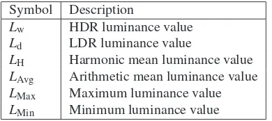
singular-ities. Note that in HDR imaging subscriptwanddrespectively refer to HDR and LDR values. The main symbols used in HDR image processing are shown in Table 2.1 for the luminance channelL.

Symbol Description

Lw HDR luminance value

Ld LDR luminance value

LH Harmonic mean luminance value

LAvg Arithmetic mean luminance value

LMax Maximum luminance value

[image:38.595.222.417.271.358.2]

LMin Minimum luminance value

Table 2.1: The main symbols used for the luminance channel.

2.2 The Generation of HDR Images

HDR content can be generated using computer graphics, photography, or an augmentation of both. Synthesising images with computer graphics takes a big effort in terms of specification of the scene. This is because each component needs to be modelled such as geometry, mate-rials, light sources, and how light is transported. On the other hand, photography is an easier process than synthesis, because a scene can be found and captured through a simple process. However, HDR content needs time consuming techniques and expensive equipment in order to be captured.

2.2.1 Synthesising HDR Images and Videos from the Virtual World

(39)

employed for rendering: ray tracing and rasterisation, see Figure 2.6.

Ray Tracing

Introduced by Whitted [219], ray tracing is a very elegant algorithm which shoots for each pixel in the screen a ray according to the direction of the camera and its lens, see Figure 2.5. This ray traverses the scene until it intersects or hits an object, which is equivalent to solving a non linear system of equations. At the hit point, the lighting is evaluated according to the material properties or BRDF, and light sources. To determine if a point is in shadow or in light, a ray is shot from the point toward the direction of the light source. Then, according to the BRDF more rays, called secondary rays, are shot in the scene to simulate reflections, refractions, inter-reflections; in general the light transport [91]. This process stops when it converges to a stable value, or when a threshold set by the user is reached.

Figure 2.5: Ray tracing: for each pixel in the image a primary ray is shot through the camera in the scene. As soon as it hits a primitive, the lighting for the hit point is evaluated. This is achieved by shooting more rays. For example, a ray towards the light is shot in the evaluation of lighting. A similar process is repeated for reflection, refractions and inter-reflections.

(40)

(a) (b)

Figure 2.6: An example of state of art of rendering quality for ray tracing and rasterisation: a) A raytraced image by by Piero Banterle using Maxwell Render from NextLimit Technologies [144]. b) A screenshot from the game Crysis by Crytek GmbH [38].

Rasterisation

Rasterisation is a different approach to solve the rendering problem compared to ray tracing. The main concept is to project each primitive that composes the scene on the screen (frame buffer) and discretise it into fragments. This operation is called scan conversion, for more detail see [66]. When a primitive is projected and discretised, visibility has to be solved to have a correct visualisation and to avoid overlaps between objects. For this task the Z-buffer [28] is generally used. The Z-buffer is an image of the same size of the frame buffer that stores depth values of previous solved fragments. For each fragment at a positionx, its depth value,F(x)z, is tested against the stored one in the Z-buffer,Z(x)z. IfF(x)z<Z(x)z, the new fragment is written in the frame buffer, andF(x)zin the Z-buffer. After the depth test, lighting is evaluated for all fragments. However, shadows, reflections, refractions, and inter-reflections are not possible to simulate natively, because rays cannot be shot. The solution is to render to a texture the scene from different positions to emulate these effects. For example, shadows are emulated by calculating a Z-buffer from the light source position, and applying a depth test during shading to determine if the point is in shadow or not [221].

(41)

many cases.

2.2.2 Capturing HDR Images and Videos from the Real World

Nowadays, available consumer cameras are limited in that they can only capture 8-bit images or 12-bit in RAW format, which do not cover the full dynamic range of irradiance values in most environments in the real world. The only way to capture HDR is to take multiple exposure images of the same scene for capturing details from the darkest to the brightest areas as proposed by Mann and Picard [123], see Figure 2.7 for an example. If the camera has a linear response, the radiance values stored in each exposure for each colour channel can be combined to recover the irradiance,E, as:

Ek(x) = ∑Ne

i=1 1

∆tiw(Ii,k(x))Ii,k(x)

∑Ni=1w(Ii,k(x))

(2.8)

where Ii is the image at the i-th exposure, k is the index of the colour channel for Ii, ∆ti is

the exposure time forIi,Neis the number of images at different exposures, andw(Ii,k(x))is a weight function that chooses pixel values to remove outliers. For example, high values can be preferred to have less noise that affects in low values. On the other hand, high values can be saturated, so middle values can be more reliable. An example of a recovered irradiance map using Equation 2.8 can be seen in Figure 2.7.f.

The problem with film and digital cameras is that they do not have a linear response, but a more general function f, called camera response function (CRF). This is due to the fact that the dynamic range of real world does not fit the medium, so as much as possible data is fitted into 8-bit or into film using f. Mann and Picard [123] proposed a simple method for calculating f, which consists of fitting the values of pixels at different exposure to a fixed CRF,

f(x) =axγ+b. This parametric f is very limited and does not support most real CRFs. Debevec and Malik [47] proposed a simple method for recovering a CRF. The value of a pixel in an image is given by the application of a CRF to the irradiance scaled by the exposure time:

(42)

(a) (b) (c) (d) (e) Lux 2.0e+00 7.7e+00 2.5e+01 7.5e+01 2.2e+02 (f)

Figure 2.7: An example of HDR capturing of the Stanford Memorial Church. Images taken with different shutter speeds: a) ₂₅₀1 sec. b) ₃₀1 sec. c) 1₄ sec. d)2sec. and e)8sec. The final HDR image obtained by combining a), b), c), d), e): f) A rendering in false colour of the luminance channel. The original HDR image is courtesy of Paul Debevec [47]

If terms are re-arranged, and a logarithm is applied to both side, the results is:

log(f−1(Ik(x))) =logEi,k(x) +log∆ti (2.10)

Assuming that f is a smooth and monotonically increasing function, f andEcan be calculated by minimising the least square error derived from Equation 2.10 using pixels from images at different exposure:

O₌

Ne

∑

i=1

sumM_j₌₁

w Ii,k(xj)

g(Ii,k(xj))−logEk(xj)−log∆ti

2

+λ

Tmax−1

∑

x=Tmin+1

(w(x)g00(x))2

(2.11)

whereg= f−1is the inverse of the CRF,Mis the number of pixel used in the minimisation, andTmaxandTminare respectively the maximum and minimum integer values in all imagesIi.

The second part of Equation 2.11 is a smoothing term for removing noise, where functionwis defined as:

w(x) =

(

x−Tmin ifx≤1₂(Tmax+Tmin)

Tmax−x ifx>1₂(Tmax+Tmin)

(2.12)

(43)

The multiple exposure method assumes that images are perfected aligned, there are no moving objects, and CCD noise is not a problem. These are very rare conditions when real world images are captured. These problems can be avoided by adapting classic alignment, ghost and noise removing techniques from image processing and computer vision, for details see [170].

HDR videos can be captured using still images, with techniques such as stop-motion or time-lapse. Nevertheless, these techniques work well in controlled scenes. To solve the video cap-turing problem Kang et al. [92] extended multiple exposure images methods to videos. The concept is to have a programmed video-camera that temporally varies the shutter speed at each frame. The final video is generated aligning and warping different frames, for combining 2 frames into a HDR one. However, the frame rate of this method is low, around 15 fps, and the scene has to contain low speed moving objects otherwise artifacts will appear. Therefore, the method is not suitable for real world situations. Nayar and Branzoi [141] developed an adaptive dynamic range camera, where a controllable liquid crystal light modulator is placed in front of the camera. This modulator adapts the exposure of each pixel on the image detector allowing to capture scenes with a very large dynamic range.

In the commercial field, a few companies provide HDR cameras based on automatic multiple exposure capturing. The two main cameras are Spheron HDR VR camera [182] by SpheronVR GmbH and Panoscan MK-3 [150] by Panoscan Ltd, which are both full 360 degree panoramic cameras at high resolution. The two cameras take full HDR images. For example, Spheron HDR VR can capture 26 f-stops of dynamic range at 50 Megapixels resolution. The develop-ment of these particular cameras was due to the necessity of quickly capturing HDR images for IBL, see Section 2.7, which is extensively used in visual effects, computer graphics, automotive and more in general for product advertising.

(44)

In the cinema industry a few companies have proposed high quality solutions such as Viper camera [189] by Thomson GV, Red One camera [167] by RED Company, and the Phantom HD camera [202] by Vision Research. All these video-cameras present high frame rates, low noise, full HD (1,920_×1,080) resolution, and a good dynamic range, 10/12-bit per channel in the logarithmic/linear domain. However, they are extremely expensive (sometimes available only for renting) and they do not fit the full dynamic range of the HVS.

2.3 Encoding HDR Images and Videos

Once HDR images/videos are captured from the real world, or they are synthesised using com-puter graphics, there is the need to store, distribute, and process these images. An uncom-pressed HDR pixel is represented using three single precision floating point numbers [82], assuming three bands as for RGB colours. This means that a pixel uses 12 bytes of memory, and an HD image 1,920_×1,080 occupies 23 Mb, an extremely large amount of space. Re-searchers have been working on compression methods for HDR content to address the high memory demands. At the beginning, only compact representations of floating point numbers were proposed, see Section 2.3.1. In the last few years, researchers have focused their efforts into more complex compression schemes, see Section 2.3.2.

2.3.1 HDR Pixels Representation in Floating Point Formats

HDR values are usually stored using single precision floating point numbers. Integer numbers, which are extensively used in LDR imaging, are not practical for storing HDR values. For example, a 32-bit unsigned integer can represent values in the range[0,232₋₁_]_{, which seems} to be enough for most HDR content. However, when a simple image processing between two or more images is carried out, for example an addition or multiplication, precision can be easily lost and overflow can occur. These are classic problems that argue in favour of floating point numbers rather than integer ones for real world values [82].

(45)

image. Ward [209] proposed the first solution to this problem, RGBE, which was meant for storing HDR values generated by the Radiance rendering system [216]. The concept is to have a shared exponent between the three colours, assuming that it does not vary much between them. The encoding of the format is defined as:

E=

log₂ max(Rw,Gw,Bw)

+128

Rm=

₂₅₆

Rw 2E−128

Gm=

₂₅₆

Gw 2E−128

Bm=

₂₅₆

Bw 2E−128

(2.13)

and the decoding as:

Rw =

Rm+0.5

256 2

E₋128 _G

w =

Gm+0.5

256 2

E₋128 _B

w =

Bm+0.5

256 2

E₋128 _(2.14)

Mantissas of the red, Rm, green, Gm, and blue, Bm, channels and the exponent, E, are then stored in an unsigned char (8-bit), achieving a final format of 32 bpp. The RGBE encoding covers 76 orders of magnitude, but the encoding does not support the full gamut of colours and negative values. To solve these problems, an image is converted to the XYZ colour space before encoding. This case is referred to as the XYZE format. Recently, the RGBE format has been implemented in graphics hardware on the NVIDIA G80 series [95], allowing very fast encoding/decoding for real-time applications.

In addition, Ward proposed a 24 and 32 bpp perceptually based format, the LogLuv format [106]. The concept is to assign more bits to luminance in the logarithmic domain than to colours in the linear domain. Firstly, an image is converted to the colour space which separates luminance (Y of XYZ) and chromaticity (CIE 1976 Uniform chromaticity(u,v)). The 32 bpp format assigns 15 bits to luminance and 16 bits to chromaticity, and it is defined as:

Le=

256(log₂Yw+64)

ue=

410u0 ve=

410v0 (2.15)

(46)

Y =2(Le+0.5)/256−64 _u0₌

1 410(ue)

v0=

1 410(ve)

(2.16)

Note that the 24 bpp format changes slightly in the constants of Equation 2.15 and Equation 2.16 according with the distribution of bits: 10 bits are allocated to luminance and 14 bits to chromaticity. While the 32 bpp format covers 38 orders of magnitude, the 24 bpp format achieves only 4.8 orders. The main advantage, over RGBE/XYZE is that the format is already in a separate colour space. Therefore, values are ready to be used for applications such as tone mapping, see Section 2.4, colour manipulation, etc.

Another important format is the half floating point format which is part of the specification of the OpenEXR file format [86]. In this representation each colour is encoded using an half precision number, which is a 16-bit implementation of the IEEE 754 standard [82], and it is defined as: H=                   

0 if M=0_∧E=0

(₋1)S₂E−15₊ M

1024 ifE=0

(₋1)S₂E−15

1+₁₀₂₄M

if 1_≤E_≤30

(₋1)S_∞ _if _E₌₃₁_∧_M₌₀

NaN if E=31_∧M>0

(2.17)

whereSis the sign, 1 bit,Mis the mantissa, 10 bits, andEis the exponent, 5 bits. Therefore, the final format is a 48 bpp, covering around 10.7 orders of magnitude. The main advantage despite the size, is that this format is implemented in graphics hardware by main vendors allowing real-time applications to use HDR images. Also, this format is considered as the de facto standard in the movie industry as the new digital negative [46].

(47)

2.3.2 HDR Image and Texture Compression

While a good floating point format can achieve down to 32/24 bpp (RGBE and LogLuv), this is not enough for distributing HDR images/videos or storing a large database of images, etc. Therefore, researchers have been working on modifying current image compression standards or proposing new methods for reducing the size of HDR images and videos. This section presents a review of the main algorithms for the compression of HDR images/videos. The focus of this review is on the compression of HDR textures, which are images used in computer graphics for increasing details of materials.

Note that some compression techniques are described in Section 3.2. These have been moved to be more coherent with the topic of Inverse Tone Mapping. These schemes are: backward compatible HDR-MPEG [125], JPEG-HDR [213, 214], HDR-JPEG 2000 [223], compression through sub-bands [115], encoding using a model of human cones [75], and two layer encoding [146].

HDR Textures Compression using Geometry Shapes

A block truncation compression (BTC) scheme [79] for HDR textures was proposed by Munkberg et al. [139]. This scheme compresses 48 bpp HDR textures into 8 bpp leveraging on logarith-mic encoding of luminance and geometry shape fitting for the chrominance channel.

The first step in the decoding scheme is to transform data in a colour space where luminance and chrominance are separated to achieve a better compression. For this task, the authors defined a colour space,Y uv, which is defined as:





Yw(x)

uw(x)

vw(x)



=



 

log₂Yw(x) 0.114_Y1

w(x)Bw(x)

0.299_Y1

w(x)Rw(x)





 Yw(x) =





0.299 0.587 0.114

  > ·  

Rw(x)

Gw(x)

Bw(x)



 (2.18)

(48)

[image:48.595.229.407.426.566.2]

(a) (b)

Figure 2.8: The encoding of chrominance in Munkberg et al. [139]: a) 2D Shapes used in the encoder. While black circles are for start and end, white circles are for interpolated values. b) An example of 2d shape fitting for a chrominance block.

other luminance values are encoded with 2 bits, which minimise the value of the interpolation betweenYminandYmax.

At this point chrominance values are compressed, the first step is to halve the resolution of the chrominance channel. For each block, a 2D shape is chosen as the one that fits chrominance values in the(u,v)plane minimising the error, see Figure 2.8. Finally, a 2 bits index is stored for each pixel which points to a sample along the fitted 2D shape.

byte 7 6 5 4 3 2 1 0

0 Ymax

1 Ymin

2 Y0 Y1 ...

...

10 typeshape ustart

11 ustart vstart

12 vstart uend

13 uend vend

14 ind0 ind1 ind2 ind3 15 ind4 ind5 ind6 ind7

Table 2.2:The table shows bits allocation for a4×4block in Munkberg et al.’s method [139].

In the decoding scheme, luminance is firstly decompressed interpolating values for each pixel in the block as:

Yw(y) = 1 3

Y_k₍_y₎Ymin+ (1−Yk(y))Ymax

(2.19)

(49)

as:

uw(y)

vw(y)

=α(ind_k₍y))

ustart−uend

vstart−vend

+β(ind_k₍y))

vend−vstart

ustart−uend

+ ustart vstart (2.20)

where α and β are parameters specific for each 2D shape. Subsequently, chrominance is up-sampled to the original size. Finally, the inverseY uvcolour space transform is applied, obtaining the reconstructed pixel:





Rw(x)

Gw(x)

Bw(x)



=2Yw(x) 



0.229−1 0.587−1 0.114−1





>



vw(x) 1₋vw(x)−uw(x)

uw(x)



 (2.21)

The compression scheme was compared against two HDR S3TC variants using mPSNR [139], log₂[RGB] RMSE [223], and HDR-VDP [127, 124]. A data set of 16 HDR textures was tested. The results showed that the method presents higher quality than S3TC variants, especially perceptually.

In conclusion the method proposed by Munkberg et al. [139] is a compression scheme that can achieve 8 bpp HDR texture compression at high quality. However, the decompression method needs special hardware, so it cannot be implemented in current graphics hardware. Furthermore, the shape fitting can take up to an hour for an one Megapixel image, which limits the scheme for fixed content.

HDR Texture Compression using Bit and Integer Operations

Co-synchronously to Munkberg et al. [139], Roimela et al. [174] presented a 8bpp BTC scheme for compressing 48 bpp HDR textures, which was later improved in Roimela et al. [175].

The first step of the coding scheme is to convert data of the texture in a colour space suitable for compression purposes. A computationally efficient colour space is defined, which splits RGB colours into luminance and chromaticity. The luminanceIw(x)is defined as:

Iw(x) = 1

4Rw(x) + 1

2Gw(x) + 1