Fault Tolerant Framework in MPI-based Distributed DEVS Simulation

Fault Tolerant Framework in MPI-based

Distributed DEVS Simulation

Bin Chen, Xiao-gang Qiu and Ke-di Huang

Abstract—Distributed DEVS simulation plays an important role in solving complex problems for its re-useability, and composability of component models. Using MPI to be the communication middleware, the distribution increases the performance. But even the tiny faults of computing resources can lead to crash. Hence Fault Tolerant is necessary to maintain the simulation reliability. This paper introduces a DEVS framework supported Fault Tolerant. The optimistic distributed simulators implement the distribution in DEVS simulation. Fault Detection, States Storage and Fault Recovery are integrated into the framework to avoid crash at runtime. Experiments are carried out to find the optimal Timeout for Fault Tolerant framework. The results indicate that the framework has to be adjusted along with the changing of simula-tion requirements. Keywords: DEVS, Fault Tolerance, Fault Detection, States Storage, Fault Recovery

1

Introduction

Discrete EVent system Specification(DEVS) has been ac-cepted as a sound formalism in modeling and simulation. The distributed protocol ofDEVShas been developed to meet the requirements for solving the particularly com-plex problems[1]. The overall simulation time can be reduced greatly because of many nodes’ participation. Many distributed frameworks are available to achieve the goal of distribution under the instructions of [2]. But even the most robust system can not maintain its reliability. So it is necessary to design a mechanism to guarantee the integration of simulation . The distribution provides the way to backup the simulation entities in case of faults. [3] presents a roll back based optimistic fault-tolerance scheme. The stable global virtual time(SGVT) is defined to make sure the safe roll back. [4] uses the buddy pro-cessor to store the copy of tasks. If the original proces-sor fails, the buddy process will be processed. [5] gives a Fault Tolerant framework based on HLA. The generic Fault Tolerant model is presented to solve the fault prob-lems in HLA-based simulations. The model is optimized on the basis of system’s features.

[3], [4] give the principles of Fault Tolerant, [6] adjust it

∗_{System Simulation Lab, School of Mechatronics and} Automa-tion, National University of Defense Technology, Changsha, China. Email: [email protected]

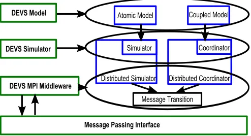
Figure 1: MPI-based Distributed DEVS Architecture

to the dynamic distributed system. [5] emphasizes the framework to solve the problems in HLA-based simula-tion. The DEVS field hasn’t been covered yet. In this paper, we provide a way to do the distribution of DEVS simulation. The distributed simulator with optimistic synchronization is introduced. Fault Detection, States Storage and Fault Recovery are discussed in detail. In section 2 we give the DEVS formalism. Section 3 in-troduces the distribution of DEVS simulation. Section 4 explains how to realize Fault Tolerant in distributed DEVS simulation. Section 5 presents the experimental data to show the improvement of distributed simulation and the optimal value for timeout. Finally, the conclusion is summarized in section 6.

2

DEVS Formalism

The DEVS formalism provides a theoretic base of model-ing the discrete event models. The formalism specifies the discrete event model in a hierarchical, modular manner. The Atomic Model, AM, is specified as follows:

AM=hX, Y, S, δint, δext, λ, tai (1)

X is the set of inputs andY is the set of outputs; S is the set of sequential states;

δint:S→S is the external state transition function; δext:Q×X→Sis the external state transition function; λ:S →Y is the output function;

ta:S→ ℜ+0 ∪ ∞is the time advance function;

Q= (s, e)|s∈S,0 =e=ta(s) is the set of total sets.

model. The coupled model could also be added into a larger coupled model according to the closure of it. The hierarchy is constructed by building coupled models. The Coupled Model, CM is defined as follows:

CM =hX, Y, D, Md, Id, Zi,d, Selecti (2)

X: a set of input events andY: a set of output events; D: a set of component references;

Md: a Classic DEVS model; Id: a set of influencees ofd;

For each iinId

Zi,d:Yi→Xd todouput translation function;

Selectis the subsets ofD→D : tie-breaking function.

3

MPI-based Distributed DEVS

Simula-tion

3.1

MPI-based Distributed DEVS

Architec-ture

In this paper, we apply Message Passing Interface(MPI) to realize distributedDEVSdistribution . MPI is seemed as the infrastructure for message communication mecha-nism. The four layer distributed architecture is shown in Figure 1. Based on theDEVSModel andDEVS Simula-tor,DEVSMPI Middleware and MPI are constructed to achieve distribution. Distributed Simulators are the key parts to add the distributed features toDEVSsimulation without touching the modeling aspect. Atomic and Cou-pled model are still simulated in the sequential simulator and coordinator. Distributed Simulator and coordina-tor collect and send the messages from sequential ones to Message Transition module. This module organizes and sends the messages to MPI. In another way, Message Transition receives the messages from MPI. Distributed simulators subsequently pass them to the sequential sim-ulators to accomplish the message circulation.

3.2

DEVS Simulator Distribution

DEVS Simulation Distribution is realized by the dis-tributed simulator. We implement optimistic disdis-tributed simulator on the basis of sequential simulator under the instructions from [7] and [8]. The Partition distributes models first, then distributed simulators are created sepa-rately on different nodes accordingly. The Root node that simulates theRoot Modelstarts and stops the simulation while all the models are connected by messages. Messages are divided into Local Message and Remote Message. Re-mote Message is used to connect models wherever they are located. Using Time Warp, optimistic simulator in-creases the simulation speed greatly.

3.2.1 Partition

Partition is the division of simulation models running in different nodes in distributed simulation. We give the definition of partition below:

P =∪Pi, N=∪Ni, i∈ {1, . . . k}, Pi= l

X

j=1

Mi,j (3)

M =

k

X

i=1

l

X

j=1

Mi,j, Mi,j ∈ {a, c} (4)

ThePi represents the partition in every simulation node Ni. M is the set of simulation models, composed ofMi,j

means the indexedj model located in theNi. Mi,j is

ei-ther the Atomic(a) or Coupled(c) model. We don’t touch the partition too much in this paper, only give the prin-ciples of partition in MPI-based Distributed DEVS Sim-ulation:

(1)∃Pr =Mr,0, Mr,0 =root(M), Root Model is the

fun-damental model in DEVS simulation, its simulator is a bit different from the common model simulator. For this reason, theNronly simulatedRoot Modelis named Root

node.

(2)∀Mi,j∈Pi, Mi,j∈ {c},∀Mi,k, Mi,j6=parentn(Mi,k),

1≤n≤depth(hierarchy). Partition does not permit the model allocated together with its parent, even the n-level parent. If the coexistence happens, it makes no sense to distribute the model. Obviously, the messaging speed inside the coordinator is much faster. When the models share the same parent are partitioned in the same node, the messages between them have to be transmitted in MPI DEVS Middle. The extra transmission slows the speed too much. And the burden on node is not relieved either.

3.2.2 Optimistic Distributed Simulator

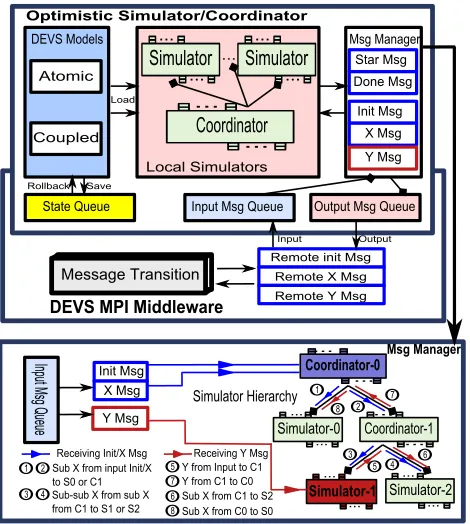
Figure 2: Fault Tolerant supported Distributed DEVS Framework

Transition wraps and unwrapps the Remote Messages. Init, X and Y messages are treated respectively due to the different message entrance in Message Manager. At runtime, the partition is published to all the simula-tion nodes, then the models are loaded. Init messages are broadcasted to all the models to the initialization. When the simulation is started, all the simulators send the local star messages to themselves to time advance. During the simulation, when the destination of the mes-sages is located remotely, the mesmes-sages are sent to DEVS MPI Middleware and store in the Output Queue. In a reverse manner, simulators inquiry DEVS MPI Middle-ware if received some messages, and store them in Input Queue. The mechanisms in Message Manager to handle the messages are different in distributed simulator and coordinator.

In distributed simulator, local simulators process the messages directly without delivery. Local star messages which lead to outputting Y messages are sent by the sim-ulator itself. There only exist the Init/X messages in Input Queue.

In distributed coordinator, the messaging process is shown in Figure 3. Message Manager transmits Init, X and Y messages to hierarchical simulators if the Input Queue is not empty, otherwise star messages are sent to local simulators to advance time. Compared to the sequential coordinator, receiving star messages have to obey the following rules.

1. The sub models located remotely are ignored in the selection of immediate star model.

2. The star messages usually lead to the Y

mes-sages from the coupled model. The Y messages are wrapped into the Remote Messages and subse-quently sent to MPI DEVS Middleware. In the mean time, they are stored in the Output Queue.

3. The termination condition has to be inquired after receiving star message in Root node.

It is worth to note that Init/X messages and Y messages are treated respectively in Message Manager. We take the three level hierarchy coordinator in Figure 3 for ex-ample. The traces in blue signify Init/X messages while the red traces represent Y messages.

If the Message Manager receives Init/X messages from Input Queue: (1) The Init/X messages arrive at Coordinator-0 first.

(2) Identified by the coupled model, the input messages are transmit to the sub simulators: Simulator-0 and Coordinator-1. If they are not the local simulator, the messages have to be wrapped into remote Init/X mes-sage and sent to relative nodes again.

(3) Coordinator-1 continues to transmit the messages to its sub simulators: simulator-1 and simulator-2. The transmission is finished when the Init/X messages cover all the local simulators.

If the Message Manager receives Y messages from Input Queue: (1) The parent simulator is found based on the parent model information in Y messages. The Figure 3 shows that Simulator-1 is the parent simulator. (2) Simulator-1 generates its own Y message by receiving in-put Y message, soon after the Simulator-1’s Y message is sent to parent Coordinator-1. (3) Coordinator-1 con-verts the Simulator-1’s Y message to be its own X mes-sage and Y mesmes-sage. X mesmes-sage is sent to Simulator-2 and 1’s Y message is sent to parent Coordinator-0. (4) Similar to Coordinator-1, Coordinator-0 converts the Y message to be its own X message and send to simulator-0. The message traces end when all the local simulators are influenced by the input Y messages.

4

Fault Tolerant in Distributed DEVS

Simulation

We introduce the design and implementation of Fault Tol-erant in this section. Even the most robust simulation system can not claim to be immune from faults. The distribution of DEVSsimulation brings the hardware re-dundancy. So it is possible to develop a framework to support Fault Tolerant.

4.1

Fault Tolerant supported Distributed

DEVS Framework

Figure 3: Distribute Simulator

Table 1: Message Channels

Channel Type Messages in Channel

Command Init, Start, Pause, Continue, Stop Detection Detect, Response, LVT, GVT Model Remote Messages

Log STas,STcc, Request

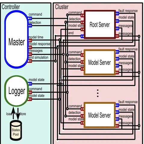
Tolerant while the servers are models’ simulation plat-forms. In addition, State Pool subordinated to Logger stores states at intervals. Master is seemed as the control center in the framework, it controls simulation’s life circle and decides when and which node is fault.

Master and Logger are connected with all the Model Servers including Root Server by message channels. The channels are constructed on MPI infrastructure. The channels are divided into Command channel, Detection channel, Model channel and Log channel. Tab 1 describes the channels and the messages in them. Command Mes-sage is used to control simulation experiments, Partition and Repartition are attached to the Init and Continue messages. Detection detects the fault nodes, GVT is at-tached to Detect message while LVT is atat-tached to Re-sponse message. Model Message is transmitted among model servers, including X-Y and anti messages. Log Message is the package within the simulator states and the request for reloading fault models. Fault Detection, States Storage and Fault Recovery are the basic elements in Fault Tolerant. We describe the algorithms and detail how they work in the framework in next sections.

Table 2: States for Storage

Entity Type State Definition Atomic Model STa=S

Atomic Simulator STas{STa, tl, tn, LV T} Coupled Model STc={Si}, Si∈ {STa, STc} Coupled Coordinator STcc{STc, tl, tn, eventList, LV T} Node STn={Si}, Si∈ {STas, STcc}

4.2

Fault Detection

We consider the faults in three categories:(1)Hardware faults to halt simulation in some node.(2)Operation Sys-tem shut down for some reason.(3)The simulator crashes. The logical faults in model and MPI-based Communi-cation faults between nodes are not covered here. And we assume that master and logger are robust enough to maintain the thousands times of simulation.

These faults cause a common phenomenon: The models on the node do not respond to any queries no matter what they are. For this reason we use detection messages to inquiry Timeout. The threshold value of Timeout is given according to specified simulation at first. Master sends detect messages to model servers periodically dur-ing simulation. If the model servers do not respond in time, the node is seemed to have been in fault.

It is important to determine the appropriate threshold value in relative simulation. If the value is larger than need, the recovery of simulation can not be activated timely. If the value is less, the false fault report causes the unnecessary recovery. Timeout differs from simula-tion to simulasimula-tion. It is not reasonable to keep the fixed value in all simulations. We do the Timeout computation by way of modeling simulation platform including simu-lation entities and Fault Tolerant entities.

These entities are built inDEVS. Simulation entities sim-ulate the protocol of Atomic Solver(simulator) model, Coordinator model and Root Coordinator model while Fault Tolerant entities are composed of Master and Log-ger Models. These DEVS models are used to load the DEVSmodels for concrete simulation applications. Once the entities and models are ready, the sequential simu-lation can be executed to compute the threshold value of Timeout. Regarded as the reference value, sequential result helps find the accurate optimal Timeout by the experiments on real system.

4.3

States Storage and Fault Recovery

in case of recovering this kind of state. Logger organizes the log messages into groups by nodes and stores them into States Pool in time order. The State Pool updates the model states as soon as the log messages are coming. Supported by Logger and State Pool, The algorithm of Fault Recovery is given below:

1. N_∗is found to having been fault by Fault Detection.

2. re partition returns Nr for reloading the fault

models.

3. ∀m_∗,j in N∗, sr′,j is created in Nr, Nr requests STas(∗, j) orSTcc(∗, j) from Logger to update sr,j. t_∗ is acquired fromsr′,j.

4. ∀si,j, i 6= r′,∀msg ∈ Qi, if t(msg) ≥ t_∗ and msg

received fromm_∗,j, si,j receives¬msg.

5. ∀si,j, i6=r′,∀msg∈Qo,ift(msg)≥t∗ and msg sent tom_∗,j, si,j sends msg tosr′,j.

The re paritition is to allocate models again to the

healthy nodes. The scheme is designed in two respects:(1) The models on the fault node are all reloaded on the chosen node. (2) The new recovering node is chosen ac-cording to the number of atomic models. On one hand, compared to the original partition, the new one does not distribute the reloading models. So the communi-cation load can remain the same level as before. On an-other hand, atomic models are in charge of most com-putation in DEVS simulation. The number of atomic models indicates the computation burden on the node.

re partition chooses the node with the least atomic

models to recover fault models.

5

Case Study and Analyze

5.1

Model Description

We build theCity Mapto model the traffic in city. The en-tities such asDistrict,Home,Office,TrafficLightController, RoadSegment and Bridge constitute the city. Car move-ment between entities is seemed as the message in im-plementation. Home, Office, TrafficLightController, Road-SegmentandBridgeare the atomic models, they are used to couple District. City Map is composed of an amount of Districtsand the RoadSegmentsor Bridgesconnecting theDistricts. At the beginning of the simulation, cars are generated in each Homes. Soon after they are transmit-ted toOfficethroughRoadSegment,TrafficLightController or Bridge. Finally, when all the cars go backHome, the simulation is terminated.

The complexity ofCity Mapis determined by the number of Districts. In order to adjust the complexity in experi-ments, we give the number in initialization.

5.2

Experiments

Supported byPython DEVS, simulators, Fault Tolerant servers and models are implemented in Pyhon. MPI is the infrastructure of distribution of simulation. There-fore MPI4Python is used to develop the distributed sim-ulators. Conservative and optimistic simulators are both implemented to show the improvement from sequential to distributed, from distributed to parallel. Our testbed is a 32 nodes cluster installed the Linux Fedora 9.0, Python 2.5, openMPI 1.2.7 and MPI4Python 1.1.0.

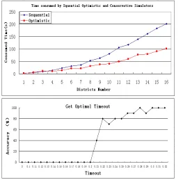
The experiments are designed in two sets: Efficiency cen-tered and Fault Tolerant cencen-tered. The former focuses on the speedup of simulators using Time Warp. The latter obtains Timeout’s optimal value for Fault Tolerant. The top picture in Fig 4 gives the consumed time curves of different number of Districts. The performance data is collected when the Districts number is 1, 2, 4, 8 and 16. Moreover, the curve in blue indicates the simulation executed on sequential simulator while the red one is the result from optimistic simulator on 2 nodes.

In another aspect, we select Timeout to do the optimiza-tion for Fault Tolerant. The Accuracy of Fault Detecoptimiza-tion is defined to help find the optimal value. The number of Districtsis 4 and the samples of Timeout are ranged from 0.0 to ∞. The experiments are performed 10 times at each point. Accuracy is the correct detection proportion in experiments.

5.3

Analyze

From the Efficiency centered experiments, it is shown that the optimistic simulator accomplishes a great deal in improving performance. The top graph shows that the consumed time approaches the half of the sequential by increasing Districtsnumber. Obviously, the performance will be elevated significantly by increasing nodes num-ber.

In the Fault Tolerant centered experiments, the Accu-racy curve indicates that the AccuAccu-racy increases from 0 to 100% along with the Timeout from 0 to∞. 100% Ac-curacy is the goal of Fault Tolerant. Simultaneously, the less the Timeout is, the better for the performance. If the Timeout is larger than necessary, lots of time is wasted in detecting faults. Therefore, the fault can not be corrected immediately, the chain faults will happen soon after. It costs much more than need for recovering the faults. In the result, the simulation performance is lowered greatly. So the value of Timeout just touches the 100% Accuracy is the most optimal one. In our experiments, the best Timeout is 0.3 second as shown in Fig 4.

6

Conclusions and Future Work

Figure 4: Experiments Results for Distribution and Timeout

framework for supporting the Fault Tolerant is designed. Fault Detection, States Storage and Fault Recovery are described respectively in advance, Master, Logger and Model Server are implemented to fulfill the requirements from Fault Tolerant. Two sets of experiments are per-formed to show the improvement of distributed DEVS simulation and the optimization for Fault Tolerant. The results testify that optimistic simulators speedup the sim-ulation a lot. And the most optimal value for Timeout is acquired at the moment Accuracy just reaches 100%. For future work, it is necessary to further the optimization in distributed simulators. The algorithms such as machine-learning have to be applied on the settings in Time Warp. They can adapt to the features in different models, hence the optimistic simulators can achieve the highest speed in all kinds of simulation. Moreover, the calibration of mod-eling simulation platforms is not limited to the Timeout. The other parameters like time delay of messages can be modeled and in consequence calculated to get the optimal value in Fault Tolerant framework.

References

[1] Fujimoto, R. M. “Parallel and distributed simulation systems,”Simulation Conference, 2001. Proceedings of the Winter, Arlington, VA, USA, pp. 147-157.

[2] Bernard. P. Zeigler, H. Praehofer, and T. G. Kim.

Theory of Modeling and Simulation, Second Edition, Academic Press, 2000.

[3] O.P. Damani and V.K. Garg, “Fault-Tolerant Dis-tributed Simulation,” Parallel and Distributed ulation, Workshop on Parallel and Distributed Sim-ulation, Los Alamitos, CA, USA, V1, pp. 3-8.

[4] Aguilar, Jose and Hern´andez, Marisela, “Fault Tol-erance Protocols for Parallel Programs Based on Tasks Replication,”MASCOTS ’00: Proceedings of the 8th International Symposium on Modeling, Anal-ysis and Simulation of Computer and Telecommuni-cation Systems, Washington. DC, USA, pp. 397-404.

[5] Dan Chen, Stephen J. Turner, Wentong Cai, “To-wards Fault-tolerant HLA-based Distributed Simu-lations,”SIMULATION, V84, N10-11, pp. 493-509.

[6] Min M., Shiyao J., Chaoqun Y., Xiaojian L., “Dy-namic Fault Tolerance in Distributed Simulation System,” Proc. International Conference on Com-putational Science (1), 2006, Reading, UK, pp.769-776.

[7] Qi L., Wainer G., “Parallel Environment for DEVS and Cell-DEVS Models,” Simulation V83, N6 pp. 449-471.