Software Reliability Estimation Based on Cubic Splines

Abstract— Software reliability is one of the most important

software quality attribute and Software reliability estimation is a hard problem to solve accurately. However for management of software quality and standard practice of the organization, accurate reliability estimation is important. Non-homogeneous Poisson Process (NHPP) models and Artificial Neural Network (ANN) models are among the most important software reliability growth models. In this paper we study an approach using past fault-related data with cubic spline Network model to estimate reliability. A numerical example is shown with simulated datasets. The example shows that the proposed model accurately estimate the software reliability.

Index Terms— Software Reliability, Cubic Spline Smoothing,

Artificial Neural Network, Software Reliability Growth Model.

I. INTRODUCTION

Software engineering is a well established discipline focused on set of management and design activities of software development. The key issues of software engineering are the management of time, cost and quality like in other engineering disciplines.

Software quality engineering comes into play prominently when the software systems grow and the impact of the software systems affect almost all in the society. Today a rapidly increasing dependency exists on the software systems. Usage of software systems can be seen in various activities ranging even to life critical systems and critical economic functions. One of the software quality issues is accuracy which is affected by errors in the software.

People are used to strike off the software systems due to software quality problems. However, when the software usage becomes mature and when the system becomes safety critical, such an attitude will not be accepted. Therefore software quality engineers are responsible to provide measurements of the quality attribute of the software system.

A. Software Quality

The term software quality has several meanings and the scope is also broadened. ISO9126 defines the software quality as: “the totality of features and characteristics of a

Manuscript received March 10, 2009. Software Reliability Estimation Based on Cubic Splines.

P. L. M. Kelani Bandara is with Vocational Training Authority of Sri Lanka, Colombo 00500, Sri Lanka and is a postgraduate student at University of Colombo School of Computing (e-mail:

[email protected]).

G. N. Wikramanayake is with University of Colombo School of Computing, Colombo 00700, Sri Lanka (e-mail: [email protected]).

J. S. Goonethillake is with University of Colombo School of Computing, Colombo 00700, Sri Lanka (e-mail: [email protected]).

software product that bear on its ability to satisfy stated or implied needs” [1].

Software quality is described in the means of models which are called software quality models and these have their own quality attributes. ISO9126 defines software quality with six software quality attributes as functionality, reliability, usability, effectiveness, maintainability and portability.

Another famous and useful categorization of factors that affect the software quality was proposed by McCall, Richards, and Walters [2]. According to that categorization, quality factors are categorized into three categories as product transition, product operation, and product revision. Software reliability is one of five product operation quality attributes.

According to the fact that the software reliability is a quality attribute in most of the quality models, it can be concluded that high quality of the software is dependent on the software reliability too. Hence if a company is to develop high quality software, it is important to employee the efforts on software reliability. In spite of this, literature state that the reliability has not been made use of with regard to the quality activities in the commercial software development [3], [4]. The following sections describe the term software reliability and why the industry doesn’t pay much attention on assurance of software reliability for their software products. In section III, a model which overcomes those problems has been proposed and finally results of our model are presented.

B. Software Reliability

IEEE defines software reliability as the ability of a program to perform required functions under stated conditions for a stated period of time [3]. Hence failures of the software reduce the reliability and to ensure the quality of the software, the measurements of the software operational failures are important. The following section describes how the reliability of the software is measured.

Software reliability is measured during the software development and during the operations using a software reliability model. There are two types of software reliability models, according to the phase which the reliability is measured.

(1) Software reliability growth model (SRGM) or software reliability estimation model — estimates the software reliability based on the observed failure data during the testing and operation phase.

(2) Software reliability prediction model — predicts the software reliability based on the reliability matrices measured or calculated during early stages of software development life cycle (prior to the integrated testing in the testing phase).

This paper focuses on the first type, the software reliability estimation model.

Software Reliability Estimation Based on Cubic

Splines

II. EXISTING SOFTWARE RELIABILITY GROWTH MODELS The first None-homogeneous Poison Process (NHPP) model, which strongly influences the development of many other models, was proposed by Goel and Okumoto [4]. Huang et al. [5] have discussed a unified scheme of discrete NHPP models by applying the concepts of weighted arithmetic, weighted geometric or weighted harmonic means. Ohba [6] presented a NHPP model with S-shaped mean value function. Lots of the generalized SRGMs, including the generalized SRGMs mentioned above, have been discussed in terms of continuous-time SRGMs, because the continuous-time SRGM is specifically applicable to the reliability analysis [7]. S. Inoue et al. give a Generalized Discrete Software Reliability Modeling based on program size [7]. Okamura et al. [8] have discussed a unified parameter estimation method based on the expectation–maximization (EM) principle and investigated the effectiveness of the estimation method based on the EM algorithm by comparing with Newton’s method [9]. Khoshgoftarr et al. [10] introduced the use of the neural networks as a tool for predicting software quality. Their model used domain metrics derived from the complexity metric data. Papers [11]-[16] have also adapted neural networks to software reliability issues. Emanm and Melo [17] have performed to construct a logistic regression model to predict which classes in a future release of a commercial Java application will be faulty.

A. Limitations of SRGMs

Even though numerous models have been discussed in literature, none is working fine in all the circumstances [18]-[19]. The most prominent limitations of the models are as the software behavior changes because the software code changes during the testing phase and hence, assumption of estimated mean time of SRGMs is violated by the dataset and more numbers of failure data are required to estimate the reliability [14], [18], [20]. Due to these limitations in SRGMs the estimation accuracy is impaired. Although this affects dramatically the reliability no attention has been given to it by the industry [18]. So it is necessary for a SRGM to overcome the above limitations in order to improve the reliability techniques used in the industry.

B. The Accuracy of Software Reliability Estimation Splines are used to interpolate a dataset to piecewise arbitrary functions which consist of third order polynomials [21], [22].

Cubic spline interpolation doesn’t assume any statistical distribution which as shown in the section II, is one of the most prominent limitations in most existing models. The software reliability is an arbitrary event and our model employee arbitrariness in several places. Pattern recognition using artificial neural network [23] makes use of randomness in its architecture when identifying an unknown pattern. That is when a new pattern is to be recognized; the artificial neural network is trained using known patterns before identifying the new pattern.

As discussed in the Section II A, the past failure dataset is usually small to make the estimation which is another limitation and that we have overcome here. To make use of our model only 9 recent failure data is needed. This solves the problem of past failure data do not show the future behavior problem discussed in Section II A.

III. SRGM WITH CUBIC SPLINES

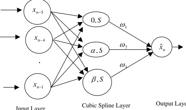
This paper gives the Artificial Neural Network (ANN) based model to capture the input–output (I/O) relationships of software systems to corresponding failures and to improve the accuracy of reliability prediction. This network captures input and output through an evolutionary algorithm.

For the input vector of

X

=

[

x

n−5

,

x

n−4

,...,

x

n−1

]

(where

n

≥

9

), the corresponding mapping of cubic spline network can be written as

x

ˆ

_n

=

g

(

x

_n−5

,

x

_n−4

,...

x

_n−1

)

.

Our model for software reliability prediction is designed as a three-layer structure with an input layer, cubic spline layer, and an output layer. Each layer has fixed nodes such as Input layer has 5 nodes corresponding to each input and cubic spline layer has 3 nodes each corresponding to the boundary conditions. The input data vector

X

is connected to the input nodes of the network to predict the time to

n

th failure.

We can derive the activation functions using cubic splines. Given a function

f

=

S

which passes through the

1 4

5

,

−

,...,

−

− n n

n

x

x

x

nodes, can be represented in splines i

S

defined on

[

x

_i−1

,

x

_i

]

where

n

−

5

≤

i

≤

n

−

1

.

∑− − =

= 1

5

n

n i Si S

A cubic spline interpolant

S

, for

f

is a function that satisfies the following six conditions,

i. The spline forms a continuous function i.e. )

1 ( ) 1 (

1 + = +

+ xi Si xi i

S for each i= n−5,n−4,...,n−2 ii. The spline forms a smooth function i.e.

)

(

)

(

_{1 1}

1 + +

+

=

′

′

_{i i i}

i

x

S

x

S

for each

2

,...,

4

,

5

−

−

−

=

n

n

n

i

iii. The second derivative is continuous i.e.

)

(

)

(

_{1 1}

1 + +

+

=

′′

′′

_{i i i}

i

x

S

x

S

for each

2

,...,

4

,

5

−

−

−

=

n

n

n

i

iv.

S

is a cubic polynomial, denoted

S

_i on subinterval

[

x

i

,

x

i+1

]

for each

i

=

n

−

5

,

n

−

4

,...,

n

−

2

v. The spline passes through each node

S

(

x

i

)

=

f

(

x

i

)

for each

i

=

n

−

5

,

n

−

4

,...,

n

−

1

vi. One of following the boundary conditions is satisfied a.

S

′′

(

x

n−5

)

=

S

′′

(

x

n−1

)

=

0

b. Set boundary derivatives for specified values.

α

=

′′

=

′′

(

x

_n−5

)

S

(

x

_n−1

)

S

c. Set boundary derivatives for specified values

β

=

′′

=

′′

(

x

n₋5

)

S

(

x

n₋1

)

S

β

α

,

are any real numbers, i.e.

−

∞

<

α

,

β

<

+∞

3 ) ( . 2 ) ( ) ( )

(X a_i b_i X x_i c_i X x_i d_i X x_i i

S = + − + − + −

for each

i

=

n

−

5

,

n

−

4

,...,

n

−

1

and

a

_i

,

b

_i

,

c

_i and

d

_i are constants.

Let

h

_i

=

x

_i+1

−

x

_i for all

i

=

n

−

5

,

n

−

4

,...,

n

−

2

The equations are simplified in finding the coefficients as follows.

i c i x

S′′( )=2* (1)

i

a i x

f( )= (2) ) 1 )( / 3 ( 1 ) 1 ( 2 1

1 − + − + + + = − −

−ci hi hi hici hi ai ai i

h (3)

i h i d i c i

c 3* *

1 = +

+ (4)

) 1 2 )( 3 / ( ) 1 )( / 1 ( ₊ − − + ₊

= h_i a_i a_i h_i c_i c_i i

b (5)

The activation function of the kth cubic spline node for estimating the nth failure is

+ − − − + − =

−_2,k(x_n) a_{n 2,k} b_{n 2,k}(x_n x_{n 2})

n S 3 ) 2 ( , 2 2 ) 2 ( ,

2 − − + − − −

− k xn xn dn k xn xn

n c

for k =1,2,3

When

k

=

1

, the boundary condition 0 ) 1 ( ) 5 ( ₋ = ′′ ₋ =

′′ x_n S x_n

S is applied.

When

k

=

2

, the boundary condition

α = − ′′ = −

′′(x_{n 5}) S(x_{n 1})

S is applied

When

k

=

3

, the boundary condition

β = − ′′ = −

′′(x_{n 5}) S(x_{n 1})

S is applied

The weight

ω

_kthat connects the kth weighting node and the output node are indicated by the weighting vectors

ω

=

[

ω

1

,

ω

2

,

ω

3

]

. These parameters are determined

by global back propagation algorithm [22].

The final output of the cubic spline networks summing layer is:

∑

= − +

= 3

1 2, ( 1)*

k Sn k Xn k

y ω

The reliability estimation of the nth failure is y

IV. RESULTS

To illustrate the proposed approach with cubic spline network model, numerical examples are studied in this section.

Table I: Time to failure data for xth failure taken from [18]. FNo

Time to

Failure FNo Time to Failure

1 20 36 21 220

2 11779 22 35580

3 40933 23 81000

4 34794 24 643095

5 17136 25 47857

6 148446 26 154800

7 7995 27 170460

8 1636 28 108540

9 15830 29 73800

10 21932 30 1860

11 2485 31 336600

12 11000 32 268140

13 2880 33 74880

14 61182 34 286200

15 4800 35 25320

16 38005 36 7080

17 16200 37 59820

18 6000 38 87900

19 1000 39 76200

20 10000 40 89280

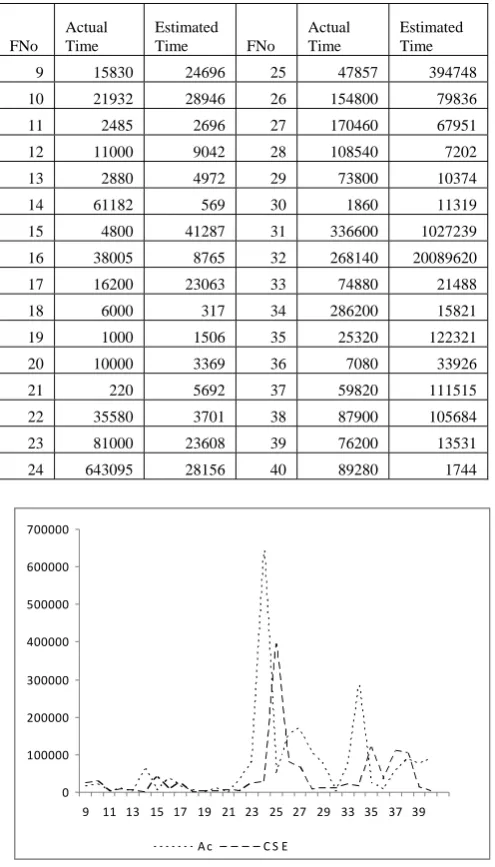
The example data of Table I is based on a project for a large Telecommunication software system [18] with FNo indicating the Failure Number for x=1...40.

Using (1)–(5) and the 3 boundary conditions in section II, the estimation of y has been done. Table II shows the estimated reliability values for our model. Validity of the estimation was checked using estimated and actual time to failure values for dataset (for x=9, 10…40). Here x commence from 9 as past 8 data is needed to estimate the parameters of our model.

S

,

0

n

x

ˆ

[image:3.595.142.442.58.235.2]

Input Layer Cubic Spline Layer Output Layer

Fig. 1: cubic spline networks

[image:4.595.42.290.84.518.2]

Table II: Actual and Estimated times for each FNo, using our model

FNo

Actual Time

Estimated

Time FNo Actual Time

Estimated Time

9 15830 24696 25 47857 394748

10 21932 28946 26 154800 79836

11 2485 2696 27 170460 67951

12 11000 9042 28 108540 7202

13 2880 4972 29 73800 10374

14 61182 569 30 1860 11319

15 4800 41287 31 336600 1027239

16 38005 8765 32 268140 20089620

17 16200 23063 33 74880 21488

18 6000 317 34 286200 15821

19 1000 1506 35 25320 122321

20 10000 3369 36 7080 33926

21 220 5692 37 59820 111515

22 35580 3701 38 87900 105684

23 81000 23608 39 76200 13531

24 643095 28156 40 89280 1744

0 100000 200000 300000 400000 500000 600000 700000

9 11 13 15 17 19 21 23 25 27 29 33 35 37 39

A c C S E

Fig. 2(a): Actual time (Ac) and estimated time using our model (CSE- Cubic Spline model Estimation) to failures.

0 200000 400000 600000 800000 1000000 1200000

9 11 13 15 17 19 21 23 25 27 29 31 34 36 38

Ac Ge JM LiL MuB

MuL Nh LiG CSE

Fig. 2(b): Comparison of estimation models with ours Fig. 2(a) compares the estimated values (Ac-Actual) using our model (CSE- Cubic Spline model Estimation) with actual time to failure data for the dataset in Table II. Fig. 2(b)

compares estimation ability of software reliability using famous models (Ac- Actual; Ge.-Geometric Model; JM -Jelinski/Morada Model; LiL - Littlewood Linear Model; MuB - Musa's Basic Model; MuL - Musa's Log Model; NHPP – None-homogeneous Poison Process Model; LiG - Littlewood Geometric Model; CSE - Cubic Splines Model).

According to the comparison, it can clearly be seen that our model and None-homogenious Poisson Process software reliability estimation model are more applicable.

The difference between actual and estimation values is lower using our model than using None-homogenious Poisson Process model.

Our model is more suitable to estimate the reliability for a dataset which doesnot have sudden deviations in the pattern (i.e. no outliers among the data values).

V. CONCLUSIONS AND FUTURE WORK

[image:4.595.43.290.87.513.2]

In this paper, we have studied an approach of reliability prediction by Cubic spline networks. Since cubic spline interpolation assumes a random distribution for the data, our model take into account the randomness. The analysis with example shows that the proposed approach works effectively. Fig. 2 indicates that our model estimation is more accurate Cubic splines interpolate a polynomial. The estimation using cubic splines can have errors upon the approximation. Since the estimation goes through weighting function in the output layer, the error component is minimized.

Since this method requires less number of input data, this can be used in the early prediction accurately.

Changing the failure behavior and the code of the software, the old data may not be valid when accounting them in reliability estimation. Recent data are only considered in our model and hence, our model improves accuracy of software reliability prediction.

However, when the dataset has outlier data such as huge increment or decrement of reliability, the estimation made using our model is less accurate. It is an identified limitation of our model.

This model contains more calculations and hence the practice of the model is tricky unless it is automated.

REFERENCES

[1] Scalet et al, “2000: ISO/IEC 9126 and 14598 integration aspects: A Brazilian viewpoint”. The Second World Congress on Software Quality, Yokohama, Japan, 2000.

[2] J.A. McCall, P.K. Richards, and G.F. Walters, “Software Quality Assurance”, 1998.

[3] A. Fries and A. Sen, “A survey of discrete Reliability-growth models.”, IEEE Trans. Rel., 45(4), 1996, pp. 582–604.

[4] A. L. Goel and K. Okumoto, "Time dependent error detection rate Model for Software Reliability and Other Performance Measures, IEEE Trans. on Rel., 28(3), 1979, pp. 206-211.

[5] C.Y. Huang, M. R. Lyu and S. Y. Kuo, “A unified Scheme of some Non-homogeneous Poisson Process models for software reliability Estimation”, IEEE Trans. Soft. Eng., 29(3), 2003, pp. 261–269. [6] S. Inoue and S. Yamada “Generalized Discrete Software Reliability

Modeling With Effect of Program Size.” IEEE Trans. on Sys., Man, and Cybernetics— Part A: Systems and Humans, 37(2), 2007, pp. 170-179.

[7] P.M. Khoshgoftaar, E.B. Allen, J.P. Hudepohl and S.J. Aud, “Application of Neural networks to software quality modeling of a very large telecommunications system”, IEEE Trans. on Neural Network, vol. 8, 1997, pp. 902-909.

[8] H. Okamura, A. Murayama, and T. Dohi, “EM Algorithm for discrete software reliability Models: A unified parameter estimation Method”, in Proc. 8th _{IEEE Int. Symp. HASE, 2004, pp. 219-228.}

[image:4.595.48.289.554.730.2]

[10] N. Karunanithi, Y. K. Malaiya, and D. Whitley, “Prediction of Software Reliability Using Neural Networks”, Proc. 1991 IEEE Int., Symp. on Soft. Rel. Eng., 1991, pp. 124-130.

[11] J.P. Hudepohl, S. J. Aud, T. M. Khoshgoftaar and E. B. Allen, et al., “EMERALD: Software Metrics and Models on the Desktop”, IEEE Soft., 13(5), 1996, pp. 56–60.

[12] K.Y. Cai, L. Cai, W. D. Wang and Z. Y. Yu, et al., “On the Neural Network Approach in Software Reliability Modeling”, The J. of Sys. and Soft., 2001, pp. 47-62.

[13] S. Yamada, and S. Osaki, “S-shaped Software Reliability Growth Model with Four Types of Software Error Data.”, Int. J. Sys. Sc., vol. 14, 1983, pp. 683-692.

[14] N. Karunanithi, D. Whitley, Y. K. Malaiya, “Using Neural Networks in Reliability Prediction”, IEEE Soft., 9(4), 1992, pp. 53-59.

[15] ANSI/AIAA, “Am. Nat’s Standard: Recommended practice for Software Reliability”, R-013-1992, Feb. 1992.

[16] S.L. Ho, M. Xie, and T.N. Goh, “A Study of the Connectionist Models for Software Reliability Prediction” Computers and Mathematics with Applications, vol. 46, 2003, pp. 1037-1045.

[17] E. Emam, and W. Melo, “The Prediction of Faulty Classes Using Object-Oriented Design Metrics”, J. of Systems and Soft., Elsevier Sc., 2001. Tec. Rep., NRCERB-1064, NRC 43609, 1999.

[18] M.R. Lyu, “Handbook of software reliability Engineering”, IEEE Comp. Soc. Press, 1996.

[19] J.A. Denton, “Accurate software reliability estimation”, Thesis of Degree of Master of Science, Colorado State University, Fort Collins, Colorado, 1999.

[20] A. Wood, “Software Reliability Growth Models”, TANDEM Tec. Rep. 96.1, Sep. 1996.

[21] B. Alford and L. Urimi, “An Analysis of various Spline Smoothing Techniques for Online Auctions, AMSC 689”, Dec. 10, 2004. [22] J.O. Ramsay, B.W. Silverman, “Functional Data Analysis”, 2nd _ed.,

Springer pub., 2005.