Abstract— Markov models are well-established stochastic models for image analysis and processing since they allow one to take into account the contextual relationships between image pixels. In this paper, we attempt to methodically review the use of Markov models and their extensions for Land Cover mapping problem in aerial imagery according to available literature and previous research works. A new Markov model combining Markov random fields and hidden Markov models and inspired from the NSHP-HMM model, initially introduced for Handwritten Words Recognition is defined. New learning and labeling procedures are derived.
Index Terms—Aerial Images, Land Cover Mapping, Markov models, Markov Random Fields MRF, Hidden Markov Models HMM.
I. INTRODUCTION
Availability of accurate and up-to-date terrain cover information is crucial to many military and public applications. For instance, land cover maps are essential inputs for Combat simulators and agricultural models.
Land cover mapping in aerial pictures can be seen as an image labeling problem since we need to assign to each pixel a missing label.
Image labeling is a topic of great importance for many computer vision systems. In general, three main approaches are used to solve computer vision problems: stochastic, structural and neural approaches. Stochastic modeling is of a great importance to solve image labeling problem; especially when there is no direct deterministic link between labels and observable pixels (two pixels sharing the same characteristics may be assigned different labels) [12]. Consequently, there is evidence that stochastic modeling is the most suited to land cover mapping given the large variations in aerial images [13].
Most stochastic systems incorporate Markov models which provide a basis for modeling contextual constraints in visual processing and interpretation.
The use of contextual information within image pixels means to go beyond the independence assumption between labels. In term of probability, the contextual constraints are expressed through local conditional probabilities.
In non-context situation (when independence assumption
Manuscript received September 17, 2008.
Mohamed El Yazid Boudaren is with the Applied Mathematics Laboratory, EMP, Algiers, Algeria (phone: +213 551 147 274; email:
Abdel Belaïd is the head of READ Group, LORIA Research Center, Vandœuvre-lès-Nancy, France (email: [email protected]).
holds) the image observation joint probability is the product of local label observation probability.
Markov models were widely used in aerial image interpretation and segmentation: land cover mapping [1, 2, 8], remote sensing [9], Coast Line detection [7] and Forest Change detection [10]. In this paper, we aim to investigate which Markov modeling could yield best results for the task of segmenting high-resolution aerial images of rural areas into its constituent cartographic objects (fields, forests, lakes…).
The rest of the paper is organized as follows: section II defines the land cover mapping problem. Section III reviews the use of several Markov models for land cover mapping. In Section IV we remind the basics of the NSHP-HMM model we defined in [3]. In section V, we define a novel Markov model combining Dependency Tree Hidden Markov Model (DT-HMM) and NSHP-MRF. Conclusion remarks and future work are discussed in the last section.
II. LAND COVER MAPPING IN AERIAL IMAGERY In this section, we formally define the so called land cover mapping problem.
Let us consider an aerial image S of sizeT = m×npixels, where m and n represent the image length and width respectively. Each pixel s∈Sis described by an observable parameter ys∈V . The symbol set V =
{
v1...vM}
may correspond to a color space or any other characteristics.The problem under consideration in this section is to allocate each of the image pixels s∈S a missed (unobservable) labelxs∈E where
{
}
N
e e
E = 1... . All
i
e are supposed beforehand known so that training can be performed on each of them taken alone. In this context, they correspond to natural object classes (fields, forests, lakes…). The problem solution consists in deriving a
class-map T
E
x∈ from a given aerial image observation y. We assume that aerial image S is of a resolution enough high that each pixel s belongs to only one natural object class.
The problem can be seen as a segmentation problem since neighboring pixels tend to belong to the same a region. The only difference is that besides segmenting the aerial image into distinguishable regions, we need to identify each region.
III. MARKOV MODELS FOR LAND COVER MAPPING A. Bayesian Naïve Segmentation
The problem resolution of the aerial image mapping described in section II can be achieved through pixelwise naïve Bayesian segmentation. This method considers each pixel taken lonely.
Let us consider a grey level aerial image of a region containing five classes: forest, grass, stone, water and sand
Markov Models and Extensions for Land Cover
Mapping in Aerial Imagery
which we denotee1,e2 ...e5respectively. Thus, for each pixel s∈S : ys and
x
s take their values inV ={
0,1...255}
andE ={
e1... e5}
respectively.In the following formulae, we will simply use
x
instead ofxsandyinstead ofyssince we assign a label to each pixel regardless of its location.The natural object class y of pixel x is chosen so that it maximizes the MAP probability.
(
)
(
( )
)
= =
∈
∈ P y
y x P y
x P x
E x E
x
, max arg max
arg *
(1) SinceP
( )
y is constant while estimating x, we only need to evaluateP(
x,y)
.(
x y)
P xE x
, max arg *
∈
= (2)
For this, we have recourse to Bayes rule.
( ) ( )
y x P x Px
E x∈
=argmax
*
(3) The probability distributions P
( )
x and P(
y x)
can be estimated from aerial images samples of the same region.( )
xP represents the proportion of the object x in the region under consideration whereas P
(
y x)
reflects the variability within the object class x.The criterion adopted here assures a minimal misclassified pixels number when the aerial image is enough big.
However, the resulting mapping when using such a method contains a lot of discontinuities. This is majorly due to noise within the image and the nature of object classes themselves. Therefore, there are justifiable reasons to think that considering grey level values of neighboring pixels when achieving the classification would improve classification accuracy. Indeed, when analyzing a pixel taken alone, it is usually impossible even for a human to tell whose class it is.
B. Local contextual Bayesian Segmentation
To surmount the problem discussed above, one can resort to estimating the object class xsof each pixels∈S using the local information
s
N
y whereNsis the neighborhood of pixel s.
(
)
= =
∈
∈ ( )
) , ( max arg max
arg *
s s s
s
s N
N s E
x N s E x s
y P
y x P y
x P
x (4)
Nevertheless, the main limit of this method is its heavy computational complexity. In fact, even for a very limited number of object classes N, one can not consider larger than an 8-Neighborhood. Since image size T is usually very big, a huge amount of local information is then overlooked when assigning labels.
Another important drawback of the previous Bayesian methods is that they do not take account of the object class repartition within the aerial image.
C. MRF Bayesian Segmentation
The MRF Bayesian segmentation overcomes the problems discussed in the previous section and enables one to take account of the geographical repartition of natural object classes while segmenting an aerial picture.
The class-map x associated to the aerial image is supposed to be the realization of an MRF.
(
xs x)
P(
xs xNs)
P S
s∈ =
∀ : (5)
It is usually computed based on the MAP criterion.
(
x y)
P x
T
E x∈
=argmax
*
(6) This is equivalent to:
(
y x) ( )
P x Px
T
E x∈
=arg max
*
(7) A particular case of Bayesian labeling consists in using the Hidden Markov Field (HMF) which assumes the following:
(
)
∏
(
)
∈
=
S s
s x
y P x
y
P (8)
(
ys x)
P(
ys xs)
P = (9)
Therefore, the likelihood probability becomes:
(
)
∏
(
)
∈
=
S s
s
s x
y P x
y
P (10)
To solve the MAP estimation problem, direct resolutions are intractable. For this reason, many approximation algorithms have been proposed. One of the most popular is ICM algorithm [11]. In [16], Pieczynski suggests to relax the assumption of noise independence by replacing
x
sbys
N
x
in the likelihood probability.(
)
∏
(
)
∈
=
S s
N
s x s
y P x
y
P (11)
However, the main drawback of HMF based classification in our opinion is that it ties a lonely pixel observation emission y to each state s x whereas one needs usually a s larger observation to decide of the class of a pixel.
Indeed, labels can be more accurately associated to regions than to solely pixels. For this reason, several works like [14] consider region-based labeling and start by segmenting the image into regions before assigning labels to pixels.
D. HMM Based Land Cover Mapping
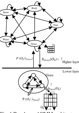
[image:2.595.361.500.491.690.2]In [1], we proposed a solution based on a hierarchical model constituted of two layers of HMM (figure 1).
Fig. 1 Two layered HMM architecture
The first layer comprises one unique HMM we called high-level HMM. It contains as many super states as the number of natural object classes. The high-level HMM models the natural objects geographical repartition. It provides us with the prior probabilityP
( )
x . Each super state is associated to a low-level HMM that models theSnow
Water
Rock
Grass
Tree
Ok
P (Ok/ λGrass) Grass
Ok ?
bGrass(Ok)
Higher layer
bGrass(Ok)= ?
P (Ok/λGrass)
corresponding object class. The low-level HMMs constitute the lower layer of the global model that provides us with the likelihood probabilityP
(
y x)
.This model principle is very similar to that of NSHP-HMM in the sense that local distributions are tied to high-level model states. The training of our two layered model has been done in two steps: firstly, the low level HMMs were trained on unitextured pictures. Secondly the high level one was trained on multitextured pictures using the parameters of HMMs of the first step, according to Baum-Welch algorithm.
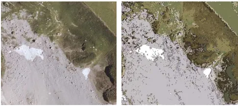
For our experiments, we used real world aerial pictures of a relatively large area, with a resolution of 50 centimeters. Our results were then used to generate reconstituted pictures like depicted in figure 2. This showed that our classifier was able to satisfactorily reproduce the original images.
[image:3.595.46.289.239.349.2]
Fig. 2 Aerial image mapping using two layered HMM model: original aerial image (left) and mapping results (right). With the permission of "Régie de Données des Pays de Savoie
RGD73-74" [17]
The main weakness of our model is that we scanned aerial images in a linear way. To weaken the repercussion of such a choice, we considered horizontal scanning within high-level HMM and vertical one within low-level models. However, numerous researches proved that 2D modeling gives better results than 1D one.
IV. COMBINING MRF AND HMM FOR HWR In [3], we proposed a particularly interesting holistic model called NSHP-HMM which advantageously combines MRF and HMM for handwritten words recognition (HWR). It is mainly based on the use of MRF at pixel level with a switching mechanism between conditional probability distributions assured by an HMM: The HMM analyzes the image columns along the writing axis and an MRF analyzes each column with specific parameters according to the current HMM state. Tying the MRF probability distributions to the HMM states enable the model to dynamically detect local features within the image (strokes of different orientations inherent to handwriting) [3].
In the present section, we briefly present the NSHP-HMM model and show how it is used to model handwritten word images.
A. NSHP-MRF (Non Symmetric Half Plane) Overview
Let L be a lattice ofn×m sites and let
{ }
( )i j L ijX
X
=
∈, be
a random field defined over the lattice L. In the context of HWR, m and n correspond to the width and length of the word image respectively and each site represents a pixel.
X
jstands for the column j of X and P(
Xij XA)
,A
⊂
L
standsforP
(
Xij Xkl)
,(
k
,
l
)
∈
A
.Finally, let us define the sets:
(
)
{
k
l
L
l
j
or
l
j
k
i
}
ij
=
∈
<
=
<
Σ
(
,
)
,
,Θ
ij⊂
Σ
ijij
Σ
is called the non-symmetric half-plane andΘ
ij the support of pixel(
i
,
j
)
∈
L
.For binarized images, the symbol setV =
{ }
0,1 . A word image is then a possible realization of a random field.X is an NSHP-MRF if and only if:
L j i X
X P X
X P
ij ij ij
ij Σ )= ( Θ )∀( , )∈
( (12)
The joint field mass probability P( X)is obtained by:
(
)
(
)
(
)
∏ ∏
∏ ∏
∏
= = Θ
= = Σ
=
−
= = =
n j
m i
ij n
j m i
ij n
j
j j
ij ij
X X P
X X P
X X X P X P
1 1 1 1
1
1 1
... , )
(
(13)
Authors usually the same form of
Θ
ijfor all pixels that is:{ }
Θij i j ∈L=
Θ ,( , )
(
)
{
i ik j jk k P jk or jk ik}
Lij= ( − , − )1≤ ≤ , >0 =0, >0 I
Θ
For instance, the pixel support may be equal to:
{
i j i j i j i j}
Lij = ( −1, −1),(, −1),( −1, ),( +1, −1) I
Θ
B. NSHP-HMM (Non-Symmetric Half-Plane Hidden Markov Model)
The key idea of NSHP-HMM is to tie the conditional probability distributions within image columns to HMM states so that these ones condition the feature sensitivity of the adjacent MRF. For instance, HMM may include specialized states to detect the presence of an upstroke or down-stroke, which would be very advantageous for HWR.
Let us rewrite the joint field mass probability in terms of pattern likelihood with respect to the HMM
λ
.(
)
∏∏
(
)
∏
= = Θ=
− =
= n
j m
i ij n
j
j j
ij
X X P X
X X P X
P
1 1
1
1
1,... , ,
)
( λ λ λ (14)
As column
X
jis associated to a parallel state stochastic processQ
=
q
1...
q
n.(
)
(
)
(
) (
)
(
) (
)
(
)
(
)
∑
∏
∏
∑
∏
∑
∑
= Θ
= −
−
= −
= =
= =
Q
m i
j ij
n j
j j
j j
j Q
n j
j j
Q Q
q X X P q
q P
q X X X P q q P
Q P Q X P Q
X P X
P
ij
1 1
1
1 1
1
1
, ,
, , ... , ,
λ λ λ λ λ
λ
(15)
Note that Q is a first order Markov process and that pixel distributions of column
X
jdepend only on the stateq
j.The results obtain by NSHP-HMM modeling on a real database of unconstrained words are extremely satisfactory. However, in opposition to other MRF based models, NSHP-HMM main weakness is the requiring of image height normalization.
V. AERIAL IMAGES MAPPING USING NSHP-HMF Our main idea was to adapt the NSHP-HMM modeling to aerial images mapping. However, unlike words images, aerial pictures do not possess a natural ordering of columns. A genuine two-dimensional modeling is then required.
of HMF methods in our opinion is that most of them assume that pixel conditional observations are independent on each other, this is more commonly called the ‘noise independence assumption’.
(
)
∏
(
)
∈
=
S s
s
s x
y P x
y
P (16)
whereP
(
ys xs)
does not depend on location s.At statexslevel, the observations inter-relationship is then ignored and a huge amount of information is then overlooked. We believe that this kind of information may be of fundamental importance in the context of aerial images mapping and propose to go beyond the noise independence assumption by linking the local observation distribution given by an NSHP-MRF to an HMF states like we did in the NSHP-HMM.
A. Non-Symmetric Half-Plane Hidden Markov Fields
Let L be a lattice of T = n×m sites and
let
{ }
( )ij L ij
X
X
=
∈, and be
Y
=
{ }
Y
ij ( )i,j∈Lthe hidden and theobservable random fields respectively of HMFλ defined over the lattice L.
In the context of images, sites correspond to pixels. n and m are image length and width respectively.
If L is a grey level image, the symbol set isV =
{
0,1..255}
.ij
X
stands for pixel state and take their values in the state setE ={
e1..eN}
. In the context of aerial images mapping, states correspond to natural object classes.ij
Y
stands for pixel( )
i, j grey-level value andP(
Yij YA)
,L
A
⊂
stands forP(
Yij Ykl)
,(
k
,
l
)
∈
A
. Finally, let us consider the sets:(
)
{
k
l
L
l
j
or
l
j
k
i
}
ij
=
∈
<
=
<
Σ
(
,
)
,
ij
ij
⊂
Σ
Θ
ij
ij
⊂
Σ
∆
where
Σ
ijis the non-symmetric half-plane andΘ
ijand∆
ij are the observable and hidden support respectively of pixel(
i
,
j
)
∈
L
.We have:
(
)
(
)
(
λ
) (
λ
)
λ
λ
X P X Y P
X Y P Y
P
X X
∑
∑
= =
, ,
(17)
(
X ,Y)
is a Non-Symmetric Half-Plane HMF (NSHP-HMF) if and only if:•
(
,λ
)
(
,λ
)
ij
X X P X
X
P ij = ij ∆ . (18)
•P
(
Yij Y,X,λ
)
P(
Yij Y ,Xij,λ
)
ij
Θ
= . (19)
B. NSHP-2D-HMM Modeling of Aerial Images
To make aerial image modeling through NSHP-HMF possible, we need to define the prior probabilityP
(
X λ)
. For this reason, we will resort in a first time to a special case of HMF models which is 2D-HMM.2D-HMM is a special case defined in a similar way to 1D-HMM. The only difference is that each state depends on one state in both horizontal and vertical directions. The causality principle is then maintained.
Let us define the state support
∆
ij:(
) (
)
{
i
j
i
j
}
L
ij
=
−
1
,
,
,
−
1
I
∆
Then, we derive the joint probability:
(
)
(
)
(
) (
)
(
)
( ) PY Y ij X P
(
X X ij)
X P X Y P
X Y P Y
P
ij
X ij L
ij ij
X X
∆
∈ Θ
∑
∏
∑
∑
= = =
,
, , , ,
λ
λ
λ
λ
λ
(20)
We only need to define
Θ
ijto make the previous formula fully defined. For instance, we can take:{
i j i j i j i j}
Lij = ( −1, −1),( , −1),( −1, ),( +1, −1) I
Θ
More explicitly, the elements of NSHP-2D HMMλ
(
A, B,Θ)
are:•
Θ
=
{ }
Θ
ij,
(
i
,
j
)
∈
L
. In this work, we consider:{
i j i j i j i j}
Lij= ( −1, −1),(, −1),( −1, ),( +1, −1) I
Θ
•
V
=
{
v
1..
v
M}
, the vocabulary of M possible symbols.∀
(
i
,
j
)
∈
L
:
Y
ij∈
V
.For instance, we can take
V
=
{
0
..
255
}
for grey-level images.•
E
=
{
e
1...
e
N}
, the set of N possible states of the model.∀
( )
i
,
j
∈
L
:
X
ij∈
E
.•
A
=
{ }
a
klm1≤k,l,m≤N,
a
klm=
P
(
X
ij=
e
mX
i−1j=
e
k,
X
ij−1=
e
l)
,the state transition matrix.
•
{
(
)
}
( )i j L N k ij
k
y
y
ijb
B
∈ ≤ ≤ Θ
=
, , 1
,
, theconditional pixel observation distribution where
(
ij) (
ij ij j k)
k
y
y
P
Y
y
Y
y
X
e
b
ij ij
ij
=
=
Θ=
Θ=
Θ
,
,
.Let us now consider the aerial image mapping problem in the NSHP-2D-HMM context: given the observation
Y
of an aerial image L and a NSHP-2D-HMMλ
(
A
, B
,
Θ
)
, mapping consists in assigning the corresponding *X that maximizes the MAP probability.
(
) ( )
(
)
( )
(
)
(
)
( ) ij ij ij ij T
ij ij
T T
X X L
j i
ij X E
x
ij L
j i
ij ij
E x
E x
a Y Y b
X X P X Y Y P
X P X Y P X
∆
∏
∏
∈ Θ
∈
∆
∈ Θ
∈ ∈
= = =
, , *
, max
arg
, , max
arg max arg
λ
(21)Where the state set
E
=
{
e
1...
e
N}
is the set of natural object classes and the symbol setV
=
{
0
..
255
}
if we consider grey-level aerial images.Finding outX*is an NP-hard problem [15]. In fact, even for classical 2D-HMM, the optimal decoding procedure is intractable in practice; contrary to 1D-HMM, the factorization of computation is not possible in 2D-HMM.
Fortunately, relaxation methods that yield good results exist in literature [4, 5]. In [5], an interesting model called Dependency Tree Hidden Markov Model (DT-HMM) was proposed to overcome the complexity problem of 2D-HMM while keeping the two-dimensional aspect of data. It is mainly based on the idea that each state depends on only one neighboring state at a time.
derive the training and recognition procedures and show that they exhibit a reasonable computational complexity.
C. DT-HMM Overview
The main idea of DT-HMM is that each state depends on only one neighboring state at the time. This neighboring state may be the horizontal or the vertical one depending on a direction random variable
t ,
( )
i
j
such that:( )
(
(
)
)
− − = 5 . 0 1 , 5 . 0 , 1 , prob with j i prob with j i j it (22)
The model assumes the following:
(
)
(
(
)
)
( ) (
( ) (
)
)
− = − = = − − ∆ 1 , , , 1 , 1 1 j i j i t if X X P j i j i t if X X P X X P j i ij H j i ij V ij ij (23) where∆
ij=
{
(
i
−
1
,
j
) (
,
i
,
j
−
1
)
}
I
L
.Let the direction function be:
( )
( ) (
( ) (
)
)
− = − = = 1 , , , 1 , , j i j i t if H j i j i t if V j iD (24)
Consequently,
(
Xij X)
PD( )i j(
Xij Xt( )i j)
P
ij = , ,
∆ (25)
The variable t defines a tree structure (dependency tree) over the lattice L with pixel (0,0) as the root.
D. DT-NSHP-HMM Definition
The DT-NSHP-HMM has the same parameters as the NSHP-2D-HMM. The only difference is in A matrix.
Horizontal and vertical states transitions are estimated separately. A matrix is then replaced by two matrices that we denote H A and V A where:
{ }
(
)
{ }
kl kl N kl(
ij l i j k)
V k ij l ij kl N l k kl H e X e X P a a A e X e X P a a A = = = = = = = = − ≤ ≤ − ≤ ≤ 1 , 1 1 , 1 , , (26) For the sake of simplicity, we will denote the DT-NSHP-HMMλ(
A, B,Θ)
where{
}
V
H A
A
A = , .
The image likelihood calculus given a dependency tree is as follows:
(
)
(
)
(
) (
)
(
)
( )(
( ))
( )∑
∏
∑
∑
∈ Θ = = =X ij L
ij j i t j i D ij X X X X X a Y Y b t X P t X Y P X Y P t Y P ij ij , , , , , , , , , ,
λ
λ
λ
λ
(27)E. Labeling Procedure
Given the observation
y
of an aerial image L and a DT-NSHP-HMMλ(
A, B,Θ)
, mapping consists in assigning the corresponding x that maximizes the MAP probability given a dependency tree function t.(
y x) ( )
P x Px
T
E x∈
=argmax
* (28)
In the following we will adapt the DT-HMM Viterbi procedure to the DT-NSHP-HMM model.
In a first time, we assume the dependency tree given. Let T
( )
i, j be the sub-tree having pixel( )
i, j as a root and letβ
i ,j( )
k be the maximum probability that YT( )i,j isgenerated starting by state k in the root
( )
i, j . Let us define:( )
( )
( ) (
) ( )
+ = = ∈ + otherwise j i j i t if l l k a j iH l E H ij
k 1 , 1 , , max
,
β
1 (29)( )
( )
( ) (
) ( )
+ = = ∈ + otherwise j i j i t if l l k a j iV l E V i j
k 1 , , 1 , max
,
β
1 (30)Thereafter, let us consider:
( )
i j H( ) ( )
i j V i jDk , = k , k , (31) We can compute the values of
β
k( )
i, j recursively as follows:( )
i j bk(
yij y k)
Dk( )
i jk , ij ,
φ
,β
= Θ (32)Finally, let us define:
( )
( )
( )
kx i j
X j i T j i T , * , , arg
β
= (33)
Note that ( )
( )
( )
k xT
X
T 0,0
* 0 , 0 0 , 0 arg
β
= is the solution of the MAP labeling defined above.
( ) * 0 , 0 * T
x
x
=
(34) Thereafter, we show how the previous algorithm can be used iteratively to produce the image labeling.According to the MAP criterion, we have:
(
)
(
)
∑
∈ ∈ ≈ = t E X E X t X Y P X Y P X T T , max arg , max arg * (35)Let us assume:
(
Y X t)
P(
Y X t)
P t t , max , ≈
∑
(36)Consequently,
(
)
{
}
(
) (
)
{
P Y X t P X t}
t X Y P X t E X t E X T T , max max arg , max max arg * ∈ ∈ ≈
≈ (37)
AsP
(
Y X,t) (
=PY X)
, therefore:(
)
(
)
{
P Y X P X t}
X t E X T max max arg * ∈
≈ (38)
Let us denote
t
P
(
X
t
)
t
max
arg
*
=
(39)We get:
(
) (
*)
* arg max P Y X,t P X t
X
T
E X∈
≈ (40)
Which we propose to solve iteratively by maximizing over t and X alternatively like follows:
(
) (
)
(
)
= = ∈ t X P t t X P X Y P X t E X T * * * * max arg max arg (41) Hence, an initialization is required to run the iterative process. We can choose either to start by initializing the dependency tree or the labeling.• Initialization: Initialize Dependency tree:
( )
(, ) (, ) ) , (min
arg
,
i j t i jj i t
y
y
j
i
t
=
−
where is Euclidian distance.
• Step 1: Achieve adapted Viterbi alignment as described above.
• Step 2: Update Dependency tree as follows:
( )
, argmax (, )( (, ), (, ))) , ( j i j i t j i D j i t x x a j i t =
• Step 3: If end criterion not reached go to step 1.
F. Training
To train our model on aerial images, we suggest performing the learning in two steps like we did in [1].
First, to compute the observations conditional probabilities, we devote an NSHP-MRF model to each natural object class. We train each model on a natural object class taken alone. Explicitly, we need to have unitextured aerial images. Then, we estimate the state transition matrix A using the parameters of the previous learned NSHP-MRF models.
Let
φ
kbe the NSHP-MRF corresponding to object class of stateek. Therefore, the classical emission probability givenby
(
)
ij
y y
bk ij, Θ is computed as follows:
(
ij) (
ij k)
k y y ij P y y ij
b , Θ = Θ ,
φ
(42)To estimate the transition matrix, we assume in a first time that we have labeled aerial pictures.
Thus, we can simply resort to a frequency-based training. Let us define the parameters:
( )
( )( )
( )
( ( ) )( )
( )
( ( ) )( )
∑
∑
∑
∈ = =
≤ ≤
∈ = =
≤ ≤
∈ = ≤
≤
− −
= = =
L j i
e x e x N
l k H
L j i
e x e x N
l k V
L j i
e x N
k
k j i t l ij
k j i t l ij k ij
l k
l k k
,
, ,
1
,
, ,
1 , 1
1 ,
, 1
1 ,
1 ,
1
ζ
ζ
ζ
(43)
We derive then the matrix A parameters as follows:
( )
( )
( )
( )
( )
( )
k l k l
k a k
l k l
k
a V
V H
H ζ
ζ ζ
ζ ,
, , ,
, = = (44)
The computational complexity order of this method is of T since we can compute the previous parameters while analyzing the image pixel by pixel, whereas the memory complexity is of
2N
2. T must be enough big to accurately model the real relationships between natural objects.If labeled images do not exist, we can estimate the state transition matrix in an iterative manner as follows:
• Initialization: Initialize transition matrix A uniformly.
• Step 1: Achieve Viterbi alignment. This provides an image labeling.
• Step 2: Re-estimate A matrix as described above.
• Step 3: If end criterion not reached go to step 1.
• End
G. Model Complexity
In this section, we demonstrate that our model exhibits a reasonable computational complexity. Let us consider a DT-NSHP-HMMλ
(
A, B,Θ)
and an aerial image L of size T. Let N be the number of states and M the number of symbols.NSHP-MRF training is performed independently on unitextured images. Since, this kind of modeling already exist, there is no need to analyze its complexity. DT-HMM modeling also already exists and it was shown in [6] that its complexity is linear with the image size T.
Accordingly, we only need to analyze our adapted Viterbi procedure. We will prove that we can convert our model to a simple DT-HMM after a set of reasonable-cost computations. If we compute for each pixel (i, j)∈L and each statek∈E the value of
(
,
)
ij
y
y
b
k ij Θ , we will have all the B matrix elements necessary to apply Viterbi procedure in a simple DT-HMM context. Consequently, the model complexity is tractable in practice.VI. CONCLUSION
In this paper, we addressed the problem of land cover mapping in aerial images. After reviewing Markov models based previous works, we reminded the NSHP-HMM formalism that we proposed in [3] for HWR and defined three new NSHP-like models.
First, we defined the NSHP-HMF which is a special case of HMF that assumes observations local conditional dependence within aerial image.
Then, we defined a particular NSHP-HMF that we called NSHP-2D-HMM which can be seen as an extension of the NSHP-HMM model since it assign a state to each image pixel instead of a whole image column.
Like HMF and 2D-HMM, direct inference methods of our new models are intractable in practice. For this reason, we proposed to approximate the NSHP-2D-HMM by a DT-NSHP-HMM that extends the DT-HMM.
REFERENCES
[1] Mohamed El Yazid Boudaren, Abdenour Labed, Adel Aziz Boulfekhar and Yacine Amara, Hidden Markov model based classification of
natural objects in aerial pictures, Proceeding of IAENG International
Conference on Signal and Image Engineering, London, July 2-4, 2008. [2] Mohamed El Yazid Boudaren, Abdenour Labed, Adel Aziz Boulfekhar and Yacine Amara, HMM based classification of natural objects in
aerial pictures, Abstract Volume of GFKL, Hamburg, Germany, July
16-18, 2008.
[3] G. Saon, A, Belaïd, High performance unconstrained word
recognition system combining HMMs and Markov random fields,
Volume 28, World Scientific, 1997.
[4] B. Merialdo, S. Marchand-Maillet, B. Huet, Approximate Viterbi
decoding for 2D-hidden Markov models, IEEE International
Conference on Acoustics, Speech and Signal Processing, Volume 6, 5-9 June 2000 , pp. 2147 – 2150.
[5] B. Merialdo, Dependency Tree Hidden Markov Models, Research Report RR-05-128, Institut Eurecom, 2005.
[6] B. Merialdo, J. Jiten, E. Galmar, B. Huet, A new approach to
probabilistic image modeling with multidimensional hidden Markov models, Adaptive multimedia retrieval 2006, pp. 95-107.
[7] Xavier Descombes, Miguel Moctezuma, Henri Maître and Jean-Paul Rudant, Coastline detection by a Markovian segmentation on SAR
images, Signal Processing, Volume 55, 1996, pp. 123-132.
[8] Teerasit Kasetkasem, Manoj K. Arora and Pramod K. Varshney,
Super-resolution land cover mapping using a Markov random field based approach, Remote Sensing of Environment, Volume 96,
Elsevier, 2005, pp. 302-314.
[9] Chi Hau Chen, Pei-Gee Peter Ho, Statistical pattern recognition in
remote sensing, Pattern Recognition, Volume 41, Elsevier, 2008, pp.
2731-2741.
[10] Desheng Liu, Kuan Song, John R. G. Townshend and Peng Gong,
Using local transition probability models in Markov random fields for forest change detection, Remote Sensing of Environment, Volume 112,
Elsevier, 2008, pp. 2222-2231.
[11] J.E. Besag, On the statistical analysis of dirty pictures (with
discussion), J. Roy. Statist. Soc. (B) 48, 1986, pp. 259–302.
[12] L. Zhang, X. Wu, An edge guided image interpolation algorithm via
directional filtering and data fusion, IEEE Transactions on Image
Processing 15 (8), 2006, pp. 2226–2238.
[13] C.M. Lai, K.M. Lam, W.C. Siu, An efficient fractal-based algorithm
for image magnification, Proceedings of the International Symposium
on Intelligent Multimedia, Video and Speech Processing, October 2004, pp. 571–574.
[14] Roger Trias Sanz, Didier Boldo, A high-reliability, high-resolution
method for land cover classification into forest and non-forest, 14th Conference on Image Analysis, Finland, 2005.
[15] E. Levin, R. Pieraccini, Dynamic planar warping for optical character
recognition, IEEE International Conference on Acoustics, Speech and
Signal Processing, Volume 3, 23-26 March 1992, pp.149 – 152. [16] Wojciech Pieczynski, Markov models in image processing, Traitement
de Signal, Volume 20 N°3, 2003, pp.255-277.