Abstract— A Finite Transfer numerical approximation
method is presented to solve a system of linear ordinary differential equations with boundary conditions. It is applied to determine the structural behaviour of the problem of a spatially curved beam element. The approach of this boundary value problem yields a unique system of differential equations. A Runge-Kutta scheme is chosen to obtain Finite Transfer expressions. The use of a recurrence strategy in these equations permits to relate both ends in the domain where boundary conditions are defined. Example of a Catenary shaped arch is provided for validation.
Index Terms— Finite Transfer Method, differential system,
boundary conditions, curved beam, Frenet-Serret formulas, transfer matrix.
I. INTRODUCTION
The problem to solve a system of linear ordinary differential equations (ODE) with boundary conditions can be approached by using analytic or numerical strategies. Being not possible to always use an exact method, approximate procedures have been resorted to [1]. In last decades, several numerical methods have arisen to solve these boundary value problems: For example, the Shooting Method [2], the Finite Difference Method [3], the Finite Element Analysis [4] and the Boundary Element Method in elasticity [5].
There exists much literature on modelling arbitrary curved beam elements [6], [7]. Traditionally, the laws governing the mechanical behaviour of a curved warped beam (applying the Euler-Bernuolli and Timoshenko theories) are defined by static equilibrium and kinematics [8], [9] or dynamic motion equations [10]. Some authors present this definition by means of compact energy equations [11], [12], [13]. These interpretations have permitted to reach accurate results, for only some types of beams: for example, a circular arch element loaded in plane [14], [15], [16], [17], [18] and loaded perpendicular to its plane [19], parabolic and elliptical beams loaded in plane [20], [21], [22] or a helix uniformly loaded [23].
Manuscript received April 21, 2008.
L. Gimena is with the Public University of Navarra, Dpt of Engineering Projects, Campus Arrosadía, Pamplona, Navarra, CP 31006, Spain (: +34 94816 9233; fax: ext. 9644; : [email protected] ).
P. Gonzaga is with the Public University of Navarra, Dpt of Engineering Projects, Campus Arrosadía, Pamplona, Navarra, CP 31006, Spain (: [email protected]).
F. Gimena is with the Public University of Navarra, Dpt of Engineering Projects, Campus Arrosadía, Pamplona, Navarra, CP 31006, Spain (: [email protected]).
In this paper, a Finite Transfer Method is proposed and applied to a system of differential equations, obtaining an incremental equation based on the transfer matrix. First, second and fourth order Runge-Kutta approximations are adopted. Using the preceding finite expression as a recurrence scheme, both extremes are related, reaching a system of algebraic equations with constant dimension regardless of the number of intervals. This boundary value problem is solved identifying the known support values in the above algebraic system. Hence, all the extremes values are determined and the recurrence scheme gives the solution at any point in the domain.
The authors focus on the arbitrary curved beam model, by means of a unique system of twelve ordinary differential equations with boundary conditions [24]. Accurate results are provided in examples for validation.
II. SYSTEMS OF DIFFERENTIAL EQUATIONS
A. System of linear ordinary differential equations of first order
Let’s define the system of ODE of first order, which represents the differential problem to solve:
1
11 1 12 2 1 1
2
21 1 22 2 2 2
1 1 2 2
p p
p p
p
p p pp p p
dx
a x
a x
a x
b
dt
dx
a x
a x
a x
b
dt
dx
a x
a x
a x
b
dt
+
+
+
+
=
+
+
+
+
=
+
+
+
+
=
K
K
M
O
M
M
K
(1)
In vector notation can be written as
( )
( )
( )
( )
d t
t
t
t
dt
=
⎡
⎣
⎤
⎦
+
x
A
x
b
(2)where
{
1 2}
( )t = x t x t( ), ( ), ,x tp( )T
x K
is the vector of the unknown functions, 11 12 1
21 22 2
1 2 ( )
p p
p p pp
a a a
a a a
t
a a a
⎡ ⎤
⎢ ⎥
⎢ ⎥
⎡ ⎤ = −
⎣ ⎦ ⎢ ⎥
⎢ ⎥
⎢ ⎥
⎣ ⎦
A
K K
M O M
K
is the matrix of variable coefficients and
{
1 2}
( )t = b b, , ,bp T
b K
is the independent vector term.
Finite Transfer Method
for the Problem of Spatially Curved Beams
B. Differential equation of order p-1.
A differential equation of p-1 order can be written as follows:
1 2
1 2 1
1 2
p p
p
p p
d
y
d
y
dy
a
a
a y
b
dt
dt
dt
− −
−
−
+
−+
K
+
+
=
(3)Making the proper change of variable:
1 1 i i i
d
y
x
dt
−−
=
fori
=
{
1, 2,
L
,
p
}
We obtain, 1 i i
dx
x
dt
+
=
fori
=
{
1, 2,
L
,
p
−
1
}
Thus, the above equation can be expressed as a fundamental system of ODE of first order:
1 2
2 3
1
1 1 2 2 1 1
0
0
0
p p p p pdx
x
dt
dx
x
dt
dx
x
dt
dx
a x
a x
a
x
b
dt
− − −−
=
−
=
−
=
+
+
+
+
=
M
O
O
M
K
(4)
In vector notation form, we reach:
( )
( )
( )
( )
d t
t
t
t
dt
=
⎡
⎣
⎤
⎦
+
x
A
x
b
(5)where
{
1 2}
( )t = x x, , ,xp T
x K is the vector of the unknown functions,
1 2 3 2 1
0 1 0 0 0 0
0 0 1 0 0 0
0 0 0 1 0 0
( )
0 0 0 1 0 0
0 0 0 0 1 0
0 0 0 0 0 1
0
p p
t
a a a a− a−
⎡ ⎤ ⎢ ⎥ ⎢ ⎥ ⎢ ⎥ ⎢ ⎥ ⎢ ⎥ ⎡ ⎤ = ⎢ ⎥ ⎣ ⎦ ⎢ ⎥ ⎢ ⎥ ⎢ ⎥ ⎢ ⎥ ⎢− − − − − ⎥ ⎣ ⎦ A K K
M M M M
K K K
is the matrix of variable coefficients, and
{
}
( )t = 0, 0, , 0,bT
b K
is independent term.
C. Analytical solution:
The analytical solution at a general point t can be expressed in function of the values at the initial point tI, as
[ ]
(
)
(
[ ]
)
( ) exp t ( ) texp t
t t t
t = dt ⎡⎢ t + − dt dt⎤⎥
⎣ ⎦
∫
I I∫
I∫
Ix A x A b (6)
Therefore, the final point tII can be related with the initial point tI with next expression:
[ ]
(
)
(
[ ])
( ) exp t ( ) t exp t
t t t
t = dt ⎡⎢ t + − dt dt⎤⎥
⎣ ⎦
∫
II∫
II∫
I I I
II I
x A x A b (7)
Boundary conditions are applied in the above formula to solve the differential system.
III. FINITE TRANSFER METHOD
Let’s establish the Finite Transfer procedure, for different order approximations.
A. Finite Transfer equation of first order.
Applying the approximation:
[ ]
( )
( )
( )
i
i i i
t
d t
t
dt
t
Δ
Δ
≅
x
=
+
x
A x
b
%
%
(8)Thus, the Finite Transfer Equation in this case is:
[ ]
[ ]
1
(
t
i+)
=
⎣
⎡
+
iΔ
t
⎤
⎦
( )
t
i+
iΔ
t
x
%
I
A
x
%
b
(9)If we use the above relation, we can write the expression of the functions at a general point ti+1 in terms of the initial point tI using a recurrence scheme
[ ]
[ ]
[ ]
1 0 0 1 ( ) ( ) j i i j j j i k ik j
j k j
t t t
t t
Δ
Δ
Δ
= + = = = = = + ⎡ ⎤ ⎡ ⎡ ⎤ ⎤ = ⎢ ⎣ +⎣ ⎦ ⎦⎥ + ⎢ ⎥ ⎣ ⎦ ⎡ ⎤ ⎡ ⎤ + ⎢ ⎣ + ⎦⎥ ⎢ ⎥ ⎣ ⎦∏
∑ ∏
Ix I A x
I A b
% %
(10)
Establishing n intervals, the two end points I (or 0) and II (or n) of the curved line will be related, where boundary conditions are applied.
[ ]
[ ]
[ ]
1 0 1 1 0 1 ( ) ( ) j n j jj n k n
k j
j k j
t t t
t t
Δ
Δ
Δ
= − = = − = − = = + ⎡ ⎤ ⎡ ⎡ ⎤ ⎤ = ⎢ ⎣ +⎣ ⎦ ⎦⎥ + ⎢ ⎥ ⎣ ⎦ ⎡ ⎤ ⎡ ⎤ + ⎢ ⎣ + ⎦⎥ ⎢ ⎥ ⎣ ⎦∏
∑ ∏
II Ix I A x
I A b
% %
(11)
We can easily demonstrate that the above expression tends in the limit to the analytical expression given in (7):
[ ] [ ]
[ ]
[ ] [ ][ ]
[ ] 1 0 0 1 10 0 1
1
0 0
1
0 0
( ) lim ( )
lim lim ( ) exp j n j t j
j n k n
k j
t j k j
j n j t j j n j k j j k k t
t t t
t t t t t t dt Δ Δ Δ Δ Δ Δ Δ Δ Δ = − → = = − = − → = = + = − → = = − = = = ⎡ ⎤ ⎡ ⎡ ⎤ ⎤ = ⎢ ⎣ +⎣ ⎦ ⎦⎥ + ⎢ ⎥ ⎣ ⎦ ⎡ ⎤ ⎡ ⎤ + ⎢ ⎣ + ⎦⎥ = ⎢ ⎥ ⎣ ⎦ ⎡ ⎤ ⎡ ⎡ ⎤ ⎤ = ⎢ ⎣ +⎣ ⎦ ⎦⎥⋅ ⎢ ⎥ ⎣ ⎦ ⎡ ⎤ ⋅⎢ + ⎥= ⎢ ⎡ + ⎤⎥ ⎣ ⎦ ⎢ ⎥ ⎣ ⎦ =
∏
∑ ∏
∏
∑
∏
II I Ix I A x
I A b
I A b x I A A % %
(
t)
( ) t exp(
t[ ])
t t
t dt dt
⎡ + − ⎤
⎢ ⎥
⎣ ⎦
∫
II∫
II∫
I I I I
x A b
(12) where, [ ]
(
[ ])
1 0 0 lim expj n t
j t
t j t dt
Δ Δ
= −
→
∏
= ⎡⎣ +⎡⎣ ⎤⎦ ⎤⎦=∫
III
I A A and,
[ ]
[ ]
[ ](
)
1 0 0 0 lim expj n t t
j
k j t t
t j k k t dt dt t Δ Δ Δ = − = → = = = − ⎡ + ⎤ ⎣ ⎦
∑
∫
∫
∏
II I I b A b I A Therefore, 0( )
lim ( )
t
t
t
Δ→
=
I I
x
x
%
and0
(
)
lim (
)
t
t
t
Δ→
=
II II
x
x
%
.Since
( )
t
I≅
( ) ; (
t
It
II)
≅
(
t
II)
B. Finite Transfer Equation for second order Runge-Kutta approximation
Applying the second order RK approximation [2]:
1 1 2
(
t
i+)
=
( ) (
t
i+
+
)
Δ
t
2
x
%
x
%
k
k
(13)Being
[ ]
1
=
i( )
t
i+
ik
A x
%
b
[
][
]
2
=
i+1( )
t
i+
1Δ
t
+
i+1k
A
x
%
k
b
Thus, the Finite Transfer Equation is:
[ ]
[
] [ ]
[
][ ]
(
)
[
]
[
]
2
1 1 1
2
1 1
( ) 2 2 ( )
2 2
( ) ( ) ( )
i i i i i i
i i i i
i i i
t t t t
t t
t t t
Δ Δ
Δ Δ
+ + +
+ +
⎡ ⎡ ⎤ ⎤
= ⎣ +⎣ + ⎦ + ⎦ +
+ + + =
= T + T
x I A A A A x
b b A b
A x b
% %
%
(14)
C. Finite Transfer Equation for fourth order RK approximation
Applying the fourth order approximation:
1 1 2 3 4
(
t
i+)
=
( ) (
t
i+
+
2
+
2
+
)
Δ
t
6
x
%
x
%
k
k
k
k
(15)Being,
[ ]
1= i ( )ti + i
k A x% b
[
]
2=⎣⎡ i+1 2⎤⎦ ( )ti + 1Δt 2 + i+1 2
k A x% k b
[
]
3=⎣⎡ i+1 2⎤⎦ ( )ti + 2Δt 2 + i+1 2
k A x% k b
[
][
]
4= i+1 ( )ti + 3Δt + i+1
k A x% k b
Thus, the Finite Transfer Equation is, in this case:
[ ]
[
]
[ ]
[
]
[ ]
[
]
[ ]
[
]
[ ]
(
)
[
]
1 1 1 2
2 2
1 1 2 1 2 1 2
2 2 3
1 1 2 1 2
2 4
1 1 2
1 1 2
1 1 2 1 2 1 2
( ) 4 6
6
12
24 ( )
4 6
i i i i
i i i i i
i i i i
i i i i
i i i
i i i i
t t
t t t t t
Δ
Δ Δ Δ
Δ
+ + +
+ + + +
+ + +
+ +
+ +
+ + + +
⎡ ⎡ ⎡ ⎤ ⎤
= ⎣ +⎣ + ⎣ ⎦+ ⎦ +
⎡ ⎡ ⎤ ⎡ ⎤ ⎡ ⎤ ⎤
+ ⎣ ⎣ ⎦ ⎣+ ⎦ +⎣ ⎦ ⎦ +
⎡ ⎡ ⎤ ⎡ ⎤ ⎤
+ ⎣ ⎣ ⎦ +⎣ ⎦ ⎦ +
⎤
⎡ ⎤
+ ⎣ ⎦ ⎦ +
+ + + +
⎡ ⎤
+ +⎣ ⎦ +
x I A A A
A A A A A
A A A A
A A A x
b b b
A b A b A
%
%
(
)
[
]
(
)
[
]
[
]
2 1 2
2 3
1 1 2 1 2 1 2
2 4
1 1 2
6
12
24
( ) ( ) ( )
i i
i i i i i
i i i
i i i
t t t
t t t
Δ Δ Δ
+
+ + + +
+ +
⎡ ⎤ +
⎣ ⎦
⎡ ⎤ ⎡ ⎤
+ ⎣ ⎦ +⎣ ⎦ +
⎡ ⎤
+ ⎣ ⎦ =
= T + T
b
A A b A b
A A b
A x% b
(16)
D. Recurrence scheme
Using one of the above Finite Transfer Equations (Eq. 9, Eq. 14 or Eq. 16), a recurrence scheme could be applied to write the expression of the functions at a general point ti+1 in
terms of the initial point tI
[
]
(
)
(
)
1
0
0 1
1 1
( ) ( ) ( ) ( ) ( )
, ( ) ,
j i j i k i
i j k j
j
j k j
i i
t t t t t
t t t t t
= = =
+
=
= = +
+ +
⎡ ⎤
⎡ ⎤
⎡ ⎤
= ⎢ ⎣ ⎦⎥ + ⎢ ⎥ =
⎢ ⎥
⎢ ⎥
⎣ ⎦ ⎣ ⎦
⎡ ⎤
= ⎣ ⎦ +
∑
∏
T I∏
T TT I I T I
x A x A b
A x b
% %
%
(17)
Establishing n intervals, the two end points I and II of the curved line are related by next equation, where the boundary conditions are applied.
[
]
(
)
(
)
1 1 1
0
0 1
( ) ( ) ( ) ( ) ( )
, ( ) ,
j n j n k n
j k j
j
j k j
t t t t t
t t t t t
= − = − = −
=
= = +
⎡ ⎤
⎡ ⎡ ⎤⎤
= ⎢ ⎣ ⎦⎥ + ⎢ ⎥ =
⎢ ⎥
⎢ ⎥
⎣ ⎦ ⎣ ⎦
= ⎡⎣ ⎤⎦ +
∑
∏
∏
II T I T T
T I II I T I II
x A x A b
A x b
% %
%
(18)
IV. DIFFERENTIAL SYSTEM FOR SPATIALLY CURVED BEAMS A curved beam is generated by a plane cross section which centroid sweeps through all the points of an axis line. The vector radius r = r(s) expresses this curved line, where s (arc length of the centroid line) is the independent variable.
The reference system used to represent the intervening known and unknown functions is the Frenet frame. Its unit vectors tangent t, normal n and binormal b are:
t
=
D
r
;n
=
D
2r
D
2r
;b
= ∧
t
n
where,
D
=
d ds
is the derivative with respect to the parameter s.The natural equations of the centroid line are expressed by the flexion curvature
χ
=
D
2r
⋅
D
2r
and the torsion curvatureτ
=
D
r
∧
(
D
2r
⋅
D
3r
) (
D
2r
⋅
D
2r
)
.The Frenet-Serret formulas are [25].
D
D
D
χ
χ
τ
τ
=
= −
+
=
−
t
n
n
t
b
b
n
(19)
Assuming the habitual principles and hypotheses (Euler-Bernuolli and Timoshenko classical beam theories) and considering the stresses associated with the normal cross-section (σ, τn, τb), the geometric characteristics of the section are: area A(s), shearing coefficients αn(s), αnb(s), αbn(s), αb(s), and moments of inertia It(s), In(s), Ib(s), Inb(s). Longitudinal E(s) and transversal G(s) elasticity moduli give the elastic condition of the material.
Applying equilibrium and kinematics laws in a differential element of the curve, the system of differential equations governing the structural behaviour of the curved beam can be obtained [24] (Equation 20 in next page bottom).
The first six rows of the system (20) represent the equilibrium equations.
The functions involved in the equilibrium equation are: Internal forces
n b
n b
A A A
N
V
V
dA
dA
dA
σ
τ
τ
+
+
=
=
∫
+
∫
+
∫
t
n
b
t
n
b
Internal moments
(
)
n b
b n
A A A
T
M
M
n
b dA
b dA
n dA
τ
τ
σ
σ
+
+
=
=
∫
−
+
∫
−
∫
t
n
b
t
n
b
Load force
q
tt
+
q
nn
+
q
bb
The last six rows of the system (20) represent the kinematics equations.
Rotations
θ
tt
+
θ
nn
+
θ
bb
Displacements
u
t
+
v
n
+
w
b
Rotation load
Θ
tt
+
Θ
nn
+
Θ
bb
Displacement load
Δ
tt
+
Δ
nn
+
Δ
bb
The differential system (Eq. 20 at the bottom page) can be annotated in vector mode as follows:
( )
( )
( )
( )
d s
s
s
s
ds
=
⎡
⎣
⎤
⎦
+
e
T
e
q
(21)Where
{
}
)
,
n,
b, ,
n,
b,
t,
n,
b, , ,
Ts
=
N V V T M
M
θ θ θ
u v w
e(
is the state vector of internal forces and deflections at a point s of the beam element, named effect in the section,
[ ] 2 2
2 2
0 0 0 0 0 0 0 0 0 0 0
0 0 0 0 0 0 0 0 0 0
0 0 0 0 0 0 0 0 0 0 0
0 0 0 0 0 0 0 0 0 0 0
0 0 1 0 0 0 0 0 0 0
0 1 0 0 0 0 0 0 0 0 0
1
0 0 0 0 0 0 0 0 0 0
0 0 0 0 0 0 0 0
)
0 0 0 0 0 0 0 0 0
1
0 0 0 0 0 0 0 0 0 0
0
t
b nb
n b nb n b nb
nb n
n b nb n b nb
GI
I I
s
E I I I E I I I
I I
E I I I E I I I
EA χ χ τ τ χ χ τ τ χ χ τ τ χ − − − − − − = ⎡ − ⎤ ⎡ − ⎤ ⎣ ⎦ ⎣ ⎦ − ⎡ − ⎤ ⎡ − ⎤ ⎣ ⎦ ⎣ ⎦ T(
0 0 0 0 0 1 0
0 0 0 0 0 1 0 0 0
n nb
bn b
GA GA
GA GA
α α χ τ
α α τ
⎡ ⎤ ⎢ ⎥ ⎢ ⎥ ⎢ ⎥ ⎢ ⎥ ⎢ ⎥ ⎢ ⎥ ⎢ ⎥ ⎢ ⎥ ⎢ ⎥ ⎢ ⎥ ⎢ ⎥ ⎢ ⎥ ⎢ ⎥ ⎢ ⎥ ⎢ ⎥ ⎢ ⎥ ⎢ ⎥ ⎢ ⎥ ⎢ − ⎥ ⎢ ⎥ ⎢ ⎥ − − ⎢ ⎥ ⎣ ⎦
is the infinitesimal Transfer Matrix, and
{
}
) t, n, b, t, n, b, t, n, b, t, n, b T
s = −q −q −q −m −m −m Θ Θ Θ Δ Δ Δ
q(
is the applied load.
A. Applying the fourth order approximation:
The approximation of the differential system (21) is given by:
1 1 2 3 4
(
s
i+)
=
( ) (
s
i+
+
2
+
2
+
)
Δ
s
6
e
%
e
%
k
k
k
k
(22)Being
[ ]
1
=
i( )
s
i+
ik
T e
%
q
[
]
2
=
⎣
⎡
i+1 2⎤
⎦
( )
s
i+
1Δ
s
2
+
i+1 2k
T
e
%
k
q
[
]
3
=
⎣
⎡
i+1 2⎤
⎦
( )
s
i+
2Δ
s
2
+
i+1 2k
T
e
%
k
q
[ ][
]
4
=
i+1( )
s
i+
3Δ
s
+
i+1k
T
e
%
k
q
Thus, the Finite Transfer Equation of four order is:
[ ]
[ ]
[ ]
[ ]
[ ]
[ ]
[ ]
[ ]
[ ]
(
)
[ ]
1 1 1 2
2 2
1 1 2 1 2 1 2
2 2 3
1 1 2 1 2
2 4
1 1 2
1 1 2
1 1 2 1 2 1 2
( ) 4 6
6
12
24 ( )
4 6
i i i i
i i i i i
i i i i
i i i i
i i i
i i i i
s s s s s s s Δ Δ Δ Δ Δ + + + + + + + + + + + + + + + + + + ⎡ ⎡ ⎡ ⎤ ⎤ = ⎣ +⎣ + ⎣ ⎦+ ⎦ + ⎡ ⎡ ⎤ ⎡ ⎤ ⎡ ⎤ ⎤ + ⎣ ⎣ ⎦ ⎣+ ⎦ +⎣ ⎦ ⎦ + ⎡ ⎡ ⎤ ⎡ ⎤ ⎤ + ⎣ ⎣ ⎦ +⎣ ⎦ ⎦ + ⎤ ⎡ ⎤ + ⎣ ⎦ ⎦ + + + + + ⎡ ⎤ + +⎣ ⎦ +
e I T T T
T T T T T
T T T T
T T T e
q q q
T q T q T
% %
(
)
[ ]
(
)
[ ]
[
]
2 1 2 2 31 1 2 1 2 1 2
2 4
1 1 2
6
12
24
( ) ( ) ( )
i i
i i i i i
i i i
i i i
s s s
s s s
Δ Δ Δ + + + + + + + ⎡ ⎤ + ⎣ ⎦ ⎡ ⎤ ⎡ ⎤ + ⎣ ⎦ +⎣ ⎦ + ⎡ ⎤ + ⎣ ⎦ =
= T + T
q
T T q T q
T T q
T e% q
(23)
Applying the recurrence scheme
[
]
(
)
(
)
1 0 0 1 1 1 ( ) ( ) ( ) ( ) ( ) , ( ) ,j i j i k i
i j k j
j
j k j
i i
s s s s s
s s s s s
= = = + = = = + + + ⎡ ⎤ ⎡ ⎡ ⎤⎤ = ⎢ ⎣ ⎦⎥ + ⎢ ⎥ = ⎢ ⎥ ⎢ ⎥ ⎣ ⎦ ⎣ ⎦ ⎡ ⎤ = ⎣ ⎦ +
∑
∏
T I∏
T TT I I T I
e T e T q
T e q
% %
%
(24)
Establishing n intervals, the two end points I and II of the curved line can be related:
[
]
(
)
(
)
1 1 1
0
0 1
( ) ( ) ( ) ( ) ( )
, ( ) ,
j n j n k n
j k j
j
j k j
s s s s s
s s s s s
= − = − = − = = = + ⎡ ⎤ ⎡ ⎤ ⎡ ⎤ = ⎢ ⎣ ⎦⎥ + ⎢ ⎥ = ⎢ ⎥ ⎢ ⎥ ⎣ ⎦ ⎣ ⎦ = ⎡⎣ ⎤⎦ +
∑
∏
∏
II T I T T
T I II I T I II
e T e T q
T e q
% %
%
(25)
Where
⎡
⎣
T s s
(
I,
II)
⎤
⎦
is the Transfer Matrix and(
,
)
T I II
q
s s
the load transfer vector [26].Finally, support conditions are applied to solve the problem.
2 2 2 2 0 0 0 0 0 0 0 0 n t
n b n
n b b
n t
b n b n
n n b b
t n t
t
n b b nb
t n b n
n b nb n b nb
n nb b n
n n b nb n b nb
DN V q
N DV V q
V DV q
DT M m
V T DM M m
V M DM m
T
D GI
M I M I
D
E I I I E I I I
M I M I
E I I I E I I I
χ χ τ τ χ χ τ τ
θ χθ Θ
χθ θ τθ Θ
τθ − + = + − + = + + = − + = − + + − + = + + + = − + − − = − − + + − − = ⎡ − ⎤ ⎡ − ⎤ ⎣ ⎦ ⎣ ⎦ − − + ⎡ − ⎤ ⎡ − ⎤ ⎣ ⎦ ⎣ ⎦ 0 0 0 0 b b t
n n nb b
b n
bn n b b
n b D N Du v EA V V
u Dv w
GA GA V V v Dw GA GA θ Θ χ Δ
α α θ χ τ Δ
α α θ τ Δ
+ − =
− − − =
− − − + + − − =
− − + + + − =
(20)
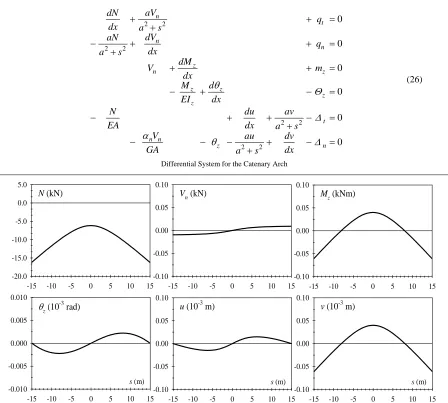
V. EXAMPLE. CATENARY SHAPED ARCHS
Parametric equations of the Catenary arch in function of the arc length, are given by:
arcsinh
x=a s a
2 2
y= + −f a a +s
Where
f
=
a
(cosh
l a
−
1)
is the height and 2l is the arch span shown in Figure 1.Vectors of the Frenet frame:
{
2 2 2 2}
, , 0
a a s s a s
= + − +
t
{
s a2 s2,a a2 s2, 0}
= + +
n b=z
Curvatures are determined:
2 2
( )s a a( s )
χ
= − + andτ
( )s =0Substituting these expressions in the general system of the spatially curved beam Eq. 20, for the case of Catenary arch loaded in plane, yields to Equation 26:
For example, we consider a uniform distributed load (udl)
q=1 kN/m. Dimensions of the arch are: f =10m; l =10m and the cross section is circular with diameter d = 0.5m.
The geometric characteristics of the section are: A = π
d.2/4, In = Ib = πd
.4
/64, and It = πd
.4
/32. Shearing deformation is neglected, thus αn=0, αz=0. The elastic isotropic homogenous material has longitudinal E = 3.107.kN/m2 and transversal G = 1,25.107.kN/m2 moduli.
Graphs of accurate results are plotted in Figure 2.
l
q
f
x
l
[image:5.612.327.526.139.293.2]y
Figure 1. Fixed-fixed udl Catenary arch.
2 2
2 2
2 2
2 2
0 0 0 0 0 0
n
t n
n z
n z
z z
z z
t n n
z n
aV dN
q
dx a s
dV aN
q dx
a s
dM
V m
dx
M d
EI dx
N du av
EA dx a s
V au dv
GA a s dx
θ Θ
Δ
α θ Δ
+ + =
+
− + + =
+
+ + =
− + − =
− + + − =
+
− − − + − =
+
(26)
Differential System for the Catenary Arch
-15 -10 -5 0 5 10 15
-0.10 -0.05 0.00 0.05 0.10
s (m)
-15 -10 -5 0 5 10 15
-0.010 -0.005 0.000 0.005 0.010
s (m)
-15 -10 -5 0 5 10 15
-0.10 -0.05 0.00 0.05 0.10
s (m)
-15 -10 -5 0 5 10 15
-0.10 -0.05 0.00 0.05 0.10
-15 -10 -5 0 5 10 15
-20.0 -15.0 -10.0 -5.0 0.0 5.0
-15 -10 -5 0 5 10 15
-0.10 -0.05 0.00 0.05 0.10
N (kN) Vn (kN) Mz (kNm)
θz (10-3 rad) u (10-3 m) v (10-3 m)
[image:5.612.82.530.322.725.2]VI. CONCLUSIONS
The exposed Finite Transfer Method solves systems of linear ordinary differential equations with boundary conditions.
It is suitable to determine the structural behaviour of the classical problem of an arbitrary curved beam element. Normally this problem is formulated in a compact energy equation form, but here the research is approached in an extended system of differential equations.
Applying a proper numerical approximation, Finite Transfer Equations are obtained. The fourth order Runge-Kutta scheme offers accurate results. It has been demonstrate how this numerical approach, tends in the limit to the analytical solution. The use of a recurrence strategy permits obtaining the Finite Transfer Equation that relates unknown functions at both extremes of the domain where boundary conditions are applied. The dimension of the resultant algebraic system is always constant and equal to the number of functions in the system, regardless of the intervals adopted, without the need of defining a mesh. The showed method is general, consistent and easy to implement in a software application.
Concerning arbitrary curved beam elements, the method presented does not distinguish between statically determinate or indeterminate beams (support conditions are applied at the end of the procedure), does not need the definition of reactions in the extremes and does not need extra formulation (virtual work principle, Castigliano’s theorems, or energy formulation). Example of a Catenary arch loaded in plane is given for verification.
REFERENCES
[1] A.P. Boresi, K.P. Chong, S. Sagal, Aproxímate solution methods in engineering mechanics. New Jersey: John Wiley & Sons; 2003. [2] R. Burden, D. Faires, Numerical Analysis. Boston: PWS, 1985. [3] M. Rahman, Applied Differential Equations for Scientists and
Engineers: Ordinary Differential Equations. Glasgow: Computational Mechanics Publications; 1991.
[4] K.J. Bathe, Finite Element Procedures. New Jersey: Prentice Hall; 1996.
[5] E. Alarcon, C. Brebbia, J. Dominguez, “The boundary element method in elasticity”. Eng Anal Bound Elem, 1978;20(9):625-639.
[6] J.I. Parcel, Moorman RB, Analysis of statically indeterminate structures. New York: John Wiley; 1955.
[7] K. Washizu, “Some considerations on a naturally curved and twisted slender beam”. J Appl Math Phys, 1964;43(2):111-116.
[8] A.E.H. Love, A Treatise on the mathematical theory of elasticity. New York: Dover; 1944.
[9] S. Timoshenko, Strength of materials. New York: D. Van Nostrand Company; 1957.
[10] H. Weiss, “Dynamics of Geometrically Nonlinear Rods: I. Mechanical Models and Equations of Motion”. Nonlinear Dynamics, 2002;30:357-381.
[11] D.L. Moris, “Curved beam stiffness coefficients”. J Struct Div
1968;94:1165-1178.
[12] V. Leontovich, Frames and arches; condensed solutions for structural analysis. New York: McGraw-Hill; 1959.
[13] H. Kardestuncer, Elementary matrix analysis of structures. New York: McGraw-Hill; 1974.
[14] Y. Yamada, Y. Ezawa, “On curved finite elements for the analysis of curved beams”. Int J Numer Meth Engng 1977;11:1635-1651. [15] D.J. Just, “Circularly curved beams under plane loads”. J Struct Div
1982;108:1858-1873.
[16] A.F. Saleeb, T.Y. Chang, “On the hybrid-mixed formulation C0 curved beam elements”. Comput Meth Appl Mech Engng 1987;60;95-121. [17] G. Shi, G.Z. Voyiadjis, “Simple and efficient shear flexible two-node
arch/beam and four-node cylindrical shell/plate finite elements”. Int J Numer Meth Engng 1991;31:759-776.
[18] L. Molari, F. Ubertini, “A flexibility-based model for linear analysis of arbitrarily curved arches”. Int J Numer Meth Engng
2006;65:1333-1353.
[19] H.P. Lee, “Generalized stiffness matrix of a curved-beam element”.
AIAA J 1969;7:2043-2045.
[20] T.M. Wang, T.F. Merrill, “Stiffness coefficients of noncircular curved beams”. J Struct Engng 1988;114:1689-1699.
[21] A. Benedetti, A. Tralli, “A new hybrid f.e. model for arbitrarily curved beam-I. Linear analysis”. Comput Struct 1989;33:1437-1449. [22] J.P. Marquis, T.M. Wang, “Stiffness matrix of parabolic beam
element”. Comput Struct 1989;6:863–870.
[23] A.C. Scordelis, “Internal forces in uniformly loaded helicoidal girders”. J Amer Conc Inst 1960;31:1013-1026.
[24] F.N. Gimena, P. Gonzaga, L. Gimena, “3D-curved beam element with varying cross-sectional area under generalized loads”. Eng Struct
2008;30:404-411.
[25] I.S. Sokolnikoff, R.M. Redeffer, Mathematics of Physics and Modern Engineering. Tokyo: McGraw-Hill; 1958.