Abstract—In this paper a novel Fourier extension based algorithm is introduced which is able to remove impulse noise from corrupted images faster than conventional algorithms. This algorithm can function faster while it preserves image details. This algorithm uses two phases, at first phase an impulse detector finds corrupted pixels and at the second phase a noise cancellation algorithm removes salt and pepper noise from the image. The results show that the proposed method is able to restore noisy pixels better than conventional algorithms and its restoration time is less than other methods making it a useful algorithm for real-time applications.
Index Terms — Image Enhancement, Impulse Noise, Nonlinear Filter.
I. INTRODUCTION
Images are usually contaminated by impulse noise while they are transmitted through communication channels or due to noisy sensors. The effect of an impulse noise on image pixels is so that the value of a pixel becomes a lot more or less than the pixels its neighborhood. It’s important to remove impulse noise before subsequent processing, such as edge detection, image segmentation and object recognition. So far different techniques are proposed to eliminate impulse noise [1]-[6], [7]-[10].
Median-based filters were amongst the first methods which attracted the attention because of their capability of preserving image edges and also because of their simplicity [5], [6]. Of course, the typical median-based filters are implemented uniformly on the image and are inclined to modify both noisy and good pixels. One way to improve this situation is to use the weighted median filter [7]-[10], an extension of the conventional median filter, which gives more weight to some values within the window around noisy pixel. It emphasizes or de-emphasizes some pixels because in most applications, some of the pixels are more important than the others. Center-weighted median (CWM) filter is the special case of the median filter [11], which gives more weight to only the central pixel of the window. It is also reasonable to give importance to the central pixel, because it is the one that has the most correlation with the desired estimate. In some recently published works a better method is introduced to enhance the restoration process which includes
Manuscript received March 31, 2008.
*
R. Rajabioun is with Control and Intelligent Processing Centre of Excellence (CIPCE), School of Electrical and Computer Engineering, University of Tehran, Tehran, Iran (Tel: +98-2182094313, Fax: +98-2188778690, Email: [email protected])
H. Sahoolizadeh is with Electrical Engineering Department, Arak Azad University, Arak, Iran (Tel: +98-7728262101, email: [email protected]).
M. Zeinali is with Electrical Engineering Department, Sahand University of Technology, Tabriz, Iran (Tel: +984123444322, e-mail: [email protected]).
a switching algorithm [2], [12]. This switching algorithm is in a way that the noisy and good pixels are separated so that the filtering algorithm changes only noisy pixels, leaving good ones unchanged. This method of filtering is called “impulse detector”.
In [1], a median-based switching filter, called progressive switching median (PSM) filter, is proposed where both the impulse detector and the noise filter are applied progressively in iterative manners. But due to its iterative manner the execution time will be noticeable and it can not be used in real-time applications. In [3], an algorithm based on long-range correlation (LRC) is introduced. This method aims to increase the range seen by conventional methods to enhance image restoration rate. Due to the fact it looks for the most similar pixel in a long range around noisy pixel, it will be necessary that the image have the property like texture. So this method will not be able to restore all kinds of images specially where there is no similar pixel to the noise disturbed one. The simulations show that this method takes a long time to finish the filtering process together with producing a poor filtered image. In [13] an adaptive rank-ordered mean (AROM) filter is proposed that employs the switching scheme based on the two-stage impulse detection mechanism. The objective is to utilize the rank-conditioned median (RCM) filter [14, 15] and CWM filter [11] to define more general operators. In the first stage of impulse detection scheme, the RCM mechanism sees if the central sample lies outside the trimming range and how much small or big the central pixel is in comparison with other pixels that lie within the trimming range in the window. In the second stage of impulse detection scheme, the CWM mechanism with variable center weights is used to decide the values of local thresholds in the sliding window. The ultimate output is switched between the current pixel itself and the rank-ordered mean of two central ranks of the surrounding pixels in the window.
Reference [16] introduces a two-phase scheme for removing salt-and-pepper impulse noise. In the first phase, an adaptive median filter is used to identify pixels which are likely to be contaminated by noise and in the second phase, the image is restored using a specialized regularization method that applies only to those selected noise candidates.
In this paper a new filtering procedure is introduced which not only removes the impulse noise from images to a great extent but also reduces the filtering time. These features make this method to be applicable to real-time applications. This algorithm works in two phases: first an impulse detector finds and flags the noise disturbed pixels and then, considering the flagged pixels, a filtering algorithm restores the noisy pixels to their original values. This algorithm works in a way that image details are preserved while impulse noise is almost fully removed. The simulation results show the
A Fourier Extension Based Algorithm for
Impulse Noise Removal
excellence of the proposed method in comparison with some conventional algorithms over different images.
Structure of rest of the paper is as follows: in section 2, impulse detection algorithm is described. Section 3 studies noise removal algorithm. Implementations and simulation are shown in section 4. Exhaustive conclusions and discussions are given in section 5.
II. IMPULSE DETECTION
Similar to other impulse detection algorithms [1-4], this impulse detector is developed by some prior information on natural images, i.e., a noise-free image should be locally smoothly varying and be separated by edges. The noise considered in this paper is only salt-and-pepper impulsive noise which means:
1) Only a proportion of all the image pixels are corrupted while other pixels are noise-free and
2) A noise pixel takes either a very large value as a positive impulse or a very small value as a negative impulse. Let xij and x ij
(new)
represent the pixel values at position (i,j) in the corrupted image and the restored image, respectively. The impulse detector generates a binary flag map where each pixel (i,j) is given a binary flag value, fij, indicating whether it
is considered as an impulse; i.e., fij =1 means the pixel in
position (i,j) is a corrupted pixel and fij = 0 means the pixel in
position (i,j) is noise free. In Sun and Neuvo’s switching I scheme they used the difference between the pixel value itself and the median value of a local window centered about it as the measurement to detect impulses. The impulse detection algorithm used here is a modified version of Sun and Neuvo’s method.
Two image sequences are generated during the impulse detection procedure [1]. The first is a sequence of gray scale images,
{{
x
ij(0)},...{
x
ij( )n},...}
, where the initial image(0)
{
x
ij}
is the noisy image to be detected,x
ij(0) denotes the pixel value at position (i,j) in the initial noisy image and( )n ij
x
is the same pixel value after nth iteration. The second is a binary flag image sequence,{{
f
ij(0)},...{
f
ij( )n},...}
, where the binary value { (n)}ij
f is used to indicate whether the pixel
at position (i,j) has been detected as an impulse, i.e., ( )
0
n ij
f =
means the pixel at position (i,j) is good pixel and ( )
1
n ij
f =
means it has been found to be an impulse. Before the first iteration, it is assumed that all the image pixels are good, i.e., (0)
0
ij
f = . In the nth iteration (n = 1, 2, ...) for each pixel
(n 1) ij
x − , the median value of the samples is found in a WD×WD (WD is an odd integer not smaller than 3) window
centered about it ( (n−1) ij
m ). The difference between (n−1)
ij
m and
) 1 (n− ij
x
provides a simple measurement to detect impulses. At first it is supposed that the image is noise free. So before the impulse detection startsf
ij(0) will be equal to zero.{
1 1 1( ) 1
(n ) (n- ) (n- ) D ij ij ij f if |x -m | T n
ij else
f
=
− <where TD is a threshold value.
When a pixel is found to be impulse noise disturbed, the value of Xij(n) is modified as follows:
{
1 11
( ) (nij ) ij(n) ij(n ) (n )
ij
n
ij
m if f f
x else
x
− −
−
≠
=
If impulse detection algorithm stops after
N
Dth iteration there will be two output images,x
ij(ND) and (ND)ij
f
. [image:2.612.349.503.198.331.2]It should be mentioned that the impulse detection measurement used here is first introduced by Sun and Neuvo in their switch I scheme [2].
Fig.1 A binary flag matrix, the same size as the original image which is R×R
pixels, used for impulse detection
III. NOISE FILTERING
To develop the algorithm proposed in this paper, following two points need to be considered: (a) as mentioned before it is assumed that the noise free image varies locally smooth and (b) a low frequency sinusoidal signal varies locally smooth too. The similarity of these two points leads to a new modeling of the image from signal processing point of view. In this paper, it is assumed that each WF×WF window of noise
free image is a sinusoidal signal which has WF components
and varies smoothly. That is, the pixel values in a WF×WF
window are assumed to be a sinusoidal signal like
0 1 2 3
( ) ( ) ( ) (2 ) ...
f t =A +ACos wt +A Sin wt +A Cos wt +
where the coefficients Ai (i=0, 1, …, WF) are obtained from
the pixel values in the window. This looks like the Fourier extension of a signal. The properties of the Fourier extension will be used to restore the noisy pixel values. For example in a noise free 3×3 window there will be maximum 9 coefficients, named Ai (i=1, 2, 3). Fig.2 gives a better sense of
[image:2.612.372.483.601.704.2]these coefficients.
Fig.2 A typical 3x3 window
a b
Fig. 3 Coefficients in a sample window around a noisy pixel used for restoration: (a) a sample flag matrix (b) the corresponding image pixels
matrix). The pixels corresponding to this flag matrix is shown in Fig. 3b. Theses pixels are noise free pixels which will be used to restore noise disturbed pixels.
As is known the Fourier extension of a signal has the RMS value of the following form:
2 2 2
2 1 2
0
... ( ( ))
2
n
A A A
RM S f t
=
A + + + +where
A
0 is the DC term and n is the number of coefficients. Due to the fact that the information of the window around noisy pixel is modeled in a sinusoidal polynomial form, the RMS of the pixel values in the window is calculated and is then restored with the value of noisy pixel. Because only the noise free pixels are used as a source to estimate corrupted pixels, A0 will be the DC term of only good pixels that can becalculated as:
0
1
1 1
n
i i
A A
n =
=
+
∑
where n is the number of good pixels in the window. So in the algorithm proposed in this paper a WF×WF sized
window is assumed around a noisy pixel of position (i,j) and then the RMS value of the assumed sinusoidal polynomial is calculated using only good pixels. Afterwards the value of impulse pixel is changed to the calculated RMS value:
( )
( ( ))
new ij
x =RMS f t
IV. IMPLEMENTATION AND SIMULATIONS
In our experiments the original test images were corrupted with fixed valued salt and pepper impulse noise, where the corrupted pixels take on the values of either 0 or 255 with equal probability. Mean Square Error (MSE) and Peak Signal to Noise Ratio (PSNR) are used to evaluate the performance of restoration algorithm. MSE is defined as:
3 3
2
1 1
1
(
ij ij)
i j
MSE
N = =
O
t
=
∑∑
−
Where N is the total number of pixels in the image while Oij
and Tij are the pixel values at position (i,j) in the original
image and test images, respectively. PSNR is defined as: 2
10
2 2
1 1
255 10 log
1
( ) ( )
r r
ij ij i j
PSNR
O T
r = =
= ×
− ∑ ∑
where r is the size of the image and Oij and Tij are the pixel
values at position (i,j) in the original image and test images, respectively. For instance in a 512×512 image r will be 512. To implement the algorithm four parameters must be
predefined. These parameters are the filtering window size, WF, the impulse detection window size, WD, the impulse
detection iteration number, ND, and the impulse detection
threshold, TD.
Due to experiments in [1], the best restoration results are obtained at values WF=3, WD=3, ND=3 and TD=40.
V. CONCLUSIONS AND DISCUSSIONS
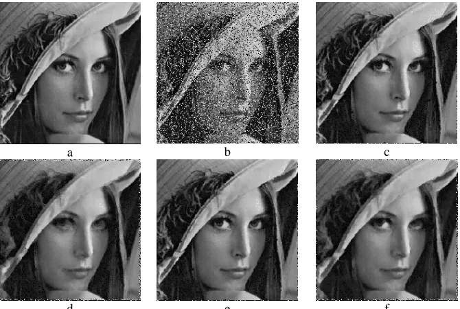
In this paper a new algorithm for impulse noise removal was introduced. This algorithm has two phases: in the first phase an impulse detector detects the noisy pixels and then, at the second phase, the noise cancellation algorithm removes salt-and-pepper impulse noise from the images. The impulse detection algorithm is a modified version of Sun and Neuvo’s Switch I scheme. Considering the properties of real noise free images and also the properties of the Fourier extension, the image is partly modeled in a sinusoidal polynomial manner. Then, using the properties of Fourier extension, the RMS value of noise free pixels are calculated and is replaced with the values of noisy pixels in each filtering window. The proposed algorithm is very fast and easy to implement. This is because there no need to any differentiation as used in [4] and also unlike some of conventional algorithms proposed in [3] does not need a large number of pixels to approximate the real value of noise disturbed pixels. Fig. 4 shows the results obtained by applying four different algorithms on “Lena” image with 25% impulse noise added to it. To demonstrate the efficiency of the proposed method in this paper, it is compared with three of the best algorithms introduced in [1], [3], [4]. Considering their results, compared with different methods, it can be concluded that these are among the best methods developed until now. So the comparison of the proposed method in this paper with these three algorithms will be meaningful.
The mentioned three algorithms are as follows: 1. Polynomial Approximation (PA) Method 2. Long Range Correlation (LRC) Method and 3. Progressive Switching Method (PSM)
Fig. 5 and Fig.6 show the MSE and PSNR values for different impulse noise values from 5% to 50%.
According to Fig. 5 and Fig. 6 it can be seen that the new algorithm proposed here in this paper has acceptable MSE and PSNR when compared with other conventional method. Fig. 7 shows the execution times of these four algorithms in compare with each other. According to Fig. 7 it can be seen that the introduced algorithm has the less execution time which together with acceptable MSE and PSNR values make it suitable for real-time applications.
a b c
d e f
Fig. 4 – (a) Original image (b) 25% fixed value noise added image (c) Proposed Algorithm (d) Long Range Correlation (LRC) Method (e) Polynomial Approximation (PA) Method (f) Progressive Switching Method
[image:4.612.139.474.46.271.2]
Fig. 5 A comparison of different median based filters’ MSE for the restoration of corrupted “Lena” image under a range of impulse noise ratio
[image:4.612.325.528.305.464.2]proposed method, i.e. PA, takes 0.1307 sec. longer (in average) to finish filtration of the noisy image. Although it might seem that this is small value but it must be considered that these values are only for gray scale images of size 512×512. When a video with large number of frames needs
Fig. 6 A comparison of different median based filters’ PSNR for the restoration of corrupted “Lena” image under a range of impulse noise ratio
Fig. 7 – Execution times of four algorithms in compare with each other
to be filtered this small value becomes a big trouble. These considerations and summaries mean that the proposed algorithm not only is able to produce acceptable results but also is able to be used in real-time applications.
TABLE 1–MSE VALUES OF FOUR FILTERING METHODS FOR WIDE RANGE OF NOISE VALUES FROM 5%-10%
Noise
Value PSM LRC PA
[image:4.612.81.288.564.720.2] [image:4.612.313.546.576.729.2]TABLE 2–PSNR VALUES OF FOUR FILTERING METHODS FOR WIDE RANGE OF NOISE VALUES FROM 5%-10%
Noise
Value PSM LRC PA
Proposed Method
5% 26.500 25.730 34.990 35.320
10% 25.950 24.690 32.960 32.740 15% 25.500 23.960 31.750 30.940 20% 24.550 22.950 29.990 29.940 25% 23.910 21.820 28.770 28.470 30% 23.510 21.370 27.430 27.170 35% 22.060 20.480 26.610 26.220 40% 21.530 19.840 25.830 24.970 50% 19.910 19.870 23.300 22.500 TABLE 3-MEAN EXECUTION TIMES FOR DIFFERENT NOISE VALUES IN
DIFFERENT RUNS
PSM LRC PA Proposed
Method 2.3551 Sec. 1.8026 Sec. 1.2431 Sec. 1.1124 Sec.
REFERENCES
[1] D. Zhang and Z. Wang, “Progressive Switching Median Filter for removal of impulse noise from highly corrupted images” IEEE Trans. on Circuits and Systems-II: Analogue and Digital Signal Processing, vol. 46, no. 1, Jan. 1999.
[2] T. Sun and Y. Neuvo “Detail-preserving median based filters in image processing”. Pattern Recognition Letters, 15:341-347, 1994. [3] Z. Wang and D. Zhang ,” Restoration of impulse noise corrupted
images using long range correlation ” IEEE Signal Processing Letters, vol. 5, no. 1, Jan. 1998.
[4] D. Zhang and Z. Wang, “Impulse noise removal using polynomial approximation” Optical Engineering, vol. 37 no. 4, April 1998. [5] D. R. K. Brownrigg, “The weighted median filter,” Commun. Ass.
Comput. Mach., vol. 27, no. 8, pp. 807–818, Aug. 1984.
[6] H. Lin and A. N. Willson, “Median filter with adaptive length,” IEEE Trans. Circuits Syst., vol. 35, pp. 675–690, June 1988.
[7] D. R. K. Brownrigg, “The weighted median filter,” Comm. ACM, vol. 27, pp. 807-818, August 1984.
[8] B. I. Justusson, “Median filtering: Statistical properties,” Two-Dimensional Digital Signal Processing II, T. S. Huang Ed., New York; Springer Verlag, 1981.
[9] T. Loupos, W. N. McDicken and P. L. Allan, “An adaptative weighted median filter for speckle suppression in medical ultrasonic images”, IEEE Trans. Circuits Syst., vol. 36, Jan. 1989.
[10] L. Yin, R. Yang, M. Gabbouj, and Y. Neuvo, “Weighted median filters: A tutorial,” IEEE Trans. Circuits and Syst. II: Analog and Digital Signal Processing, vol. 43, pp. 157-192, Mar. 1996.
[11] S-J. Ko and Y. H. Lee, “Center-weighted median filters and their applications to image enhancement,” IEEE Trans. Circuits and Syst., vol. 38, pp. 984-993, Sept. 1991.
[12] D. Zhang and Z. Wang, “Impulse noise detection and removal using fuzzy techniques,” Electron. Lett., vol. 33, pp. 378–379, Feb. 1997. [13] K. M. Singh, P.K. Bora, S.B. Singh, “Adaptive Rank-ordered Mean
Filter for Removal of Impulse Noise from Images”, IEEE International Conference on Industrial Technology, vol. 2, pp. 980-985, 2002. [14] R. C. Hardie and K. E. Barner, “Rank-conditioned rank selection filters
for signal restoration,” IEEE Trans. Image Processing, vol. 2, no. 2, pp. 192-206, Mar. 1994.
[15] L. Alparone, S. Baronti and R. Carlà, “ Two-Dimensional rank-conditioned median filter,” IEEE Trans. on Circuits and Systems – II: Analog and Digital Signal Processing, vol. 42, No. 2, Feb. 1995. [16] Find this: R.H. Chan, H. Chung-Wa, M. Nikolova, “Salt-and-Pepper
Noise Removal by Median-Type Noise Detectors and Detail-Preserving Regularization”, IEEE Transactions on image Processing, vol. 14, No. 10, pp. 1479-1485,2005.
[17] I. Pitas and A. N. Venetsanopoulos, Nonlinear Digital Filters: Principles and Applications. Boston, MA: Kluwer, 1990.
[18] D. R. K. Brownrigg, “The weighted median filter,” Commun. Ass. Comput. Mach., vol. 27, no. 8, pp. 807–818, Aug. 1984.
[19] H. Lin and A. N. Willson, “Median filter with adaptive length,” IEEE Trans. Circuits Syst., vol. 35, pp. 675–690, June 1988.
[20] E. Abreu, M. Lightstone, S. K. Mitra, and K. Arakawa, “A new efficient approach for the removal of impulse noise from highly corrupted images,” IEEE Trans. Image Processing, vol. 5, pp. 1012-1025, June 1996.
[21] D. Zhang and Z. Wang, “Impulse noise detection and removal using fuzzy techniques,” Electron. Lett. , vol. 33, pp. 378–379, Feb. 1997. [22] H. M. Lin and A. N. Willson, “Median filters with adaptive length,”
IEEE Trans. Circuits Syst., vol. 35, pp. 675–690, June 1988. [23] E. Abreu, M. Lightstone, S. K. Mitra, and K. Arakawa, “A new
efficient approach for the removal of impulse noise from highly corrupted images,” IEEE Trans. Image Processing, vol. 5, pp. 1012-1025, June 1996.