A Semiparametric Model for Bayesian Reader Identification
Ahmed Abdelwahab1 and Reinhold Kliegl2 and Niels Landwehr1 1 Department of Computer Science, Universit¨at Potsdam
August-Bebel-Straße 89, 14482 Potsdam, Germany {ahmed.abdelwahab, niels.landwehr}@uni-potsdam.de
2Department of Psychology, Universit¨at Potsdam Karl-Liebknecht-Straße 24/25, 14476 Potsdam OT/Golm
Abstract
We study the problem of identifying individu-als based on their characteristic gaze patterns during reading of arbitrary text. The motiva-tion for this problem is an unobtrusive biomet-ric setting in which a user is observed during access to a document, but no specific chal-lenge protocol requiring the user’s time and at-tention is carried out. Existing models of indi-vidual differences in gaze control during read-ing are either based on simple aggregate fea-tures of eye movements, or rely on paramet-ric density models to describe, for instance, saccade amplitudes or word fixation durations. We develop flexible semiparametric models of eye movements during reading in which den-sities are inferred under a Gaussian process prior centered at a parametric distribution fam-ily that is expected to approximate the true dis-tribution well. An empirical study on read-ing data from 251 individuals shows signifi-cant improvements over the state of the art.
1 Introduction
Eye-movement patterns during skilled reading con-sist of brief fixations of individual words in a text that are interleaved with quick eye movements calledsaccadesthat change the point of fixation to another word. Eye movements are driven both by low-level visual cues and high-level linguistic and cognitive processes related to text understanding; as a reflection of the interplay between vision, cog-nition, and motor control during reading they are frequently studied in cognitive psychology (Kliegl et al., 2006; Rayner, 1998). Computational mod-els (Engbert et al., 2005; Reichle et al., 1998) as well
as models based on machine learning (Matties and Søgaard, 2013; Hara et al., 2012) have been devel-oped to study how gaze patterns arise based on text content and structure, facilitating the understanding of human reading processes.
A central observation in these and earlier psycho-logical studies (Huey, 1908; Dixon, 1951) is that eye movement patterns strongly differ between individu-als. Holland et al. (2012) and Landwehr et al. (2014) have developed models of individual differences in eye movement patterns during reading, and studied these models in a biometric problem setting where an individual has to be identified based on observing her eye movement patterns while reading arbitrary text. Using eye movements during reading as a bio-metric feature has the advantage that it suffices to observe a user during a routine access to a device or document, without requiring the user to react to a specific challenge protocol. If the observed eye movement sequence is unlikely to be generated by an authorized individual, access can be terminated or an additional verification requested. This is in con-trast to approaches where biometric identification is based on eye movements in response to an artificial visual stimulus, for example a moving (Kasprowski and Ober, 2004; Komogortsev et al., 2010; Rigas et al., 2012b; Zhang and Juhola, 2012) or fixed (Bed-narik et al., 2005) dot on a computer screen, or a specific image stimulus (Rigas et al., 2012a).
The model studied by Holland & Komogort-sev (2012) uses aggregate features (such as average fixation duration) of the observed eye movements. Landwehr et al. (2014) showed that readers can be identified more accurately with a model that cap-tures aspects of individual-specific distributions over
eye movements, such as the distribution over fixa-tion durafixa-tions or saccade amplitudes for word refix-ations, regressions, or next-word movements. Some of these distributions need to be estimated from very few observations; a key challenge is thus to design models that are flexible enough to capture character-istic differences between readers yet robust to sparse data. Landwehr et al. (2014) used a fully paramet-ric approach where all densities are assumed to be in the gamma family; gamma distributions were shown to approximate the true distribution of interest well for most cases (see Figure 1). This model is robust to sparse data, but might not be flexible enough to capture all differences between readers.
The model we study in this paper follows ideas developed by Landwehr et al. (2014), but em-ploys more flexible semiparametric density models. Specifically, we place a Gaussian process prior over densities that concentrates probability mass on den-sities that are close to the gamma family. Given data, a posterior distribution over densities is de-rived. If data is sparse, the posterior will still be sharply peaked around distributions in the gamma family, reducing the effective capacity of the model and minimizing overfitting. However, given enough evidence in the data, the model will also deviate from the gamma-centered prior—depending on the kernel function chosen for the GP prior, any density function can in principle be represented. Integrating over the space of densities weighted by the posterior yields a marginal likelihood for novel observations from which predictions are inferred. We empirically study this model in the same setting as studied by Landwehr et al. (2014), but using an order of mag-nitude more individuals. Identification error is re-duced by more than a factor of three compared to the state of the art.
The rest of the paper is organized as follows. After defining the problem setting in Section 2, Section 3 presents the semiparametric probabilis-tic model. Section 4 discusses inference, Section 5 presents an empirical study on reader identification.
2 Problem Setting
Assume R different readers, indexed by r ∈
{1, . . . , R}, and letX ={X1, . . . ,Xn}denote a set
of texts. Eachr ∈ Rgenerates a set of eye
move-ment patternsS(r)={S1(r), . . . ,S(nr)}onX, by
S(ir)∼p(S|Xi, r,Γ)
wherep(S|Xi, r,Γ)is a reader-specific distribution
over eye movement patterns given a textXi. Here, r is a variable indicating the reader generating the sequence, andΓ is a true but unknown model that defines all reader-specific distributions. We assume thatΓcan be broken down into reader-specific mod-els,Γ= (γ1, . . . ,γk), such that the distribution
p(S|Xi, r,Γ) =p(S|Xi,γr) (1)
is defined by the partial modelγr. We aggregate the
observations of all readers on the training data into a variableS(1:R)= (S(1), . . . ,S(R)).
We follow a Bayesian approach, defining a prior
p(Γ)over the joint model that factorizes into priors over reader-specific models, p(Γ) = QRr=1p(γr).
At test time, we observe novel eye movement patterns S¯ = {S¯1, . . . ,S¯m} on a novel set of textsX¯ ={X¯1, . . . ,X¯m}generated by an unknown
reader r ∈ R. We assume a uniform prior over
readers, that is, each r ∈ Ris equally likely to be observed at test time. The goal is to infer the most likely reader to have generated the novel eye move-ment patterns. In a Bayesian setting, this means in-ferring the most likely reader given the training ob-servations (X,S(1:R)) and test observation (X¯,S¯):
r∗= arg max
r∈Rp(r|
¯
X,S¯,X,S(1:R)). (2)
We can rewrite Equation 2 to
r∗ = arg max
r∈Rp( ¯S|r,
¯
X,X,S(1:R)) (3)
= arg max
r∈R Z
p( ¯S|r,X¯,Γ)p(Γ|X,S(1:R))dΓ
= arg max
r∈R Z
p( ¯S|X¯,γr)p(γr|X,S(r))dγr (4)
where
p( ¯S|X¯,γr) = m Y
i=1
p(¯Si|X¯i,γr) (5)
p(γr|X,S(r))∝p(γr) n Y
i=1
In Equation 3 we exploit that readers are uniformly chosen at test time, and in Equation 4 we exploit the factorization p(Γ) = QRr=1p(γr) of the prior,
which together with Equation 1 entails a factoriza-tion p(Γ|X,S(1:R)) = QR
r=1p(γr|X,S(r)) of the
posterior. Note that Equation 4 states that at test time we predict the readerr for which the marginal
likelihood (that is, after integrating out the reader-specific model γr) of the test observations is
high-est. The next section discusses the reader-specific modelsp(S|X,γr)and prior distributionsp(γr).
3 Probabilistic Model
The probabilistic model we employ follows the gen-eral structure proposed by Landwehr et al. (2014), but employs semiparametric density models and al-lows for fully Bayesian inference. To reduce nota-tional clutter, let γ ∈ {γ1, . . . ,γR} denote a
par-ticular reader-specific model, and let X ∈ X de-note a text. An eye movement pattern is a sequence S = ((s1, d1), . . . ,(sT, dT))of gaze fixations,
con-sisting of a fixation positionst(position in text that
was fixated) and durationdt ∈R(length of fixation
in milliseconds). In our experiments, individual sen-tences are presented in a single line on screen, thus we only model a horizontal gaze positionst ∈ R.
We modelp(S|X,γ)as a dynamic process that suc-cessively generates fixation positions st and
dura-tionsdtinS, reflecting how a reader generates a
se-quence of saccades in response to a text stimulusX:
p(S|X,γ) =p(s1, d1|X,γ) T Y
t=2
p(st, dt|st−1,X,γ),
wherep(st, dt|st−1,X,γ)models the generation of
the next fixation position and duration given the old fixation position st−1. In the psychological
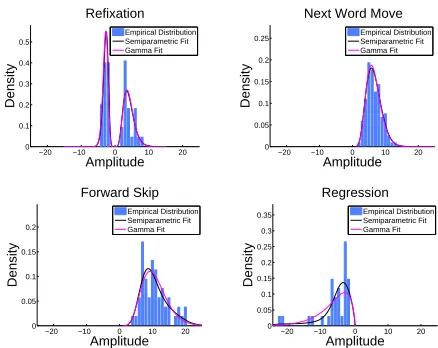
litera-ture, four differentsaccade types are distinguished: a reader can refixate the current word (refixation), fixate the next word in the text (next word move-ment), move the fixation to a word after the next word, that is, skip one or more words (forward skip), or regress to fixate a word occurring earlier in the text (regression), see, e.g., Heister et al. (2012). We observe empirically that for each saccade type, there is a characteristic distribution over saccade am-plitudes and fixation durations, and that both ap-proximately follow gamma distributions—see
Fig-−20 −10 0 10 20 0
0.1 0.2 0.3 0.4 0.5
Density
Amplitude Refixation
Empirical Distribution Semiparametric Fit Gamma Fit
−20 −10 0 10 20 0
0.05 0.1 0.15 0.2 0.25
Density
Amplitude Next Word Move
Empirical Distribution Semiparametric Fit Gamma Fit
−20 −10 0 10 20 0
0.05 0.1 0.15 0.2
Density
Amplitude Forward Skip
Empirical Distribution Semiparametric Fit Gamma Fit
−20 −10 0 10 20 0
0.05 0.1 0.15 0.2 0.25 0.3 0.35
Density
Amplitude Regression
[image:3.612.311.530.57.231.2]Empirical Distribution Semiparametric Fit Gamma Fit
Figure 1: Empirical distributions of saccade amplitudes in training data for first individual, with fitted Gamma distribu-tions and semiparametric distribution fits.
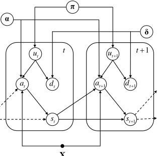
ure 1. We therefore modelp(st, dt|st−1,X,γ)
us-ing a mixture over distributions for the four different saccade types. At each timet, the model first draws
a saccade type ut∈ {1,2,3,4}, and then draws a
saccade amplitudeat and fixation durationdtfrom
type-specific distributions p(a|ut, st−1,X,γ) and p(d|ut,γ). More formally,
ut∼p(u|π) (7) at∼p(a|ut, st−1,X,α) (8) dt∼p(d|ut,δ), (9)
where γ = (π,α,δ) is decomposed into compo-nentsπ,α, and δ. Afterwards, the model updates
the fixation position according to st=st−1+at,
concluding the definition of p(st, dt|st−1,X,γ).
Figure 2 shows a slice in the dynamical model. The distribution p(u|π) over saccade types (Equation 7) is multinomial with parameter vector
π ∈ R4. The distributions over amplitudes and
du-rations (Equations 8 and 9) are modeled semipara-metrically as discussed in the following subsections.
3.1 Model of Saccade Amplitudes
We first discuss the amplitude model
p(a|ut, st−1,X,α) (Equation 8). We first
de-fine a distribution p(a|ut,α) over amplitudes for
saccade type ut, and subsequently discuss
t
u ut1
t
a dt at1 dt1
t t1
X
t
s st1
π α
[image:4.612.106.263.59.214.2]δ
Figure 2:Plate notation of of a slice in the dynamic model.
leading top(a|ut, st−1,X,α). We define
p(a|ut= 1,α) = (
µα1(a) :a >0
(1−µ)¯α1(−a) :a≤0
(10)
whereµis a mixture weight andα1,α¯1are densities
defining the distribution over positive and negative amplitudes for the saccade typerefixation, and
p(a|ut= 2,α) =α2(a) (11) p(a|ut= 3,α) =α3(a) (12) p(a|ut= 4,α) =α4(−a) (13)
whereα2(a),α3(a), and α4(a) are densities
defin-ing the distribution over amplitudes for the remain-ing saccade types. Finally, the distribution
p(s1|X,α) =α0(s1) (14)
over the initial fixation position is given by another density function α0. The variables µ, α0, α1, α¯1, α2, α3, andα4 are aggregated into model
compo-nentα. For resolving the most likely reader at test
time (Equation 4), densities inαwill be integrated
out under a prior based on Gaussian processes (Sec-tion 3.3) using MCMC inference (Sec(Sec-tion 4).
Given the old fixation position st−1, the text X,
and the chosen saccade type ut, the amplitude is
constrained to fall within a specific interval. For in-stance, for a refixation the amplitude has to be cho-sen such that the novel fixation position lies within the beginning and the end of the currently fixated word; a regression implies an amplitude that is neg-ative and makes the novel fixation position lie be-fore the beginning of the currently fixated word.
These constraints imposed by the text structure de-fine the conditional distributionp(a|ut, st−1,X,α).
More formally, p(a|ut, st−1,X,α) is the
distribu-tionp(a|ut,α)conditioned ona∈[l, r], that is,
p(a|ut, st−1,X,α) =p(a|a∈[l, r], ut,α),
wherelandr are the minimum and maximum
am-plitude consistent with the constraints. Recall that for a distribution over a continuous variablexgiven by densityα(x), the distribution overxconditioned
onx∈[l, r]is given by the truncated density
α(x|x∈[l, r]) =
( α(x)
Rr
l α(¯x)d¯x
:x∈[l, r]
0 :x /∈[l, r]. (15)
We derivep(a|ut, st−1,X,α)by truncating the
dis-tributions given by Equations 10 to 13 to the min-imum and maxmin-imum amplitude consistent with the current fixation position st−1 and text X. Let wl◦
(w◦r) denote the position of the left-most (right-most) character of the currently fixated word, and letwl+, wr+denote these positions for the next word
inX. Let furthermorel◦=wl◦−st−1,r◦ = w◦r− st−1,l+ =w+l −st−1, andr+=w+r −st−1. Then
p(a|ut= 1, st−1,X,α) = (
µα1(a|a∈[0, r◦]) :a >0
(1−µ)¯α1(−a|a∈[l◦,0]) :a≤0
(16)
p(a|ut= 2, st−1,X,α) =α2(a|a∈[l+, r+]) (17) p(a|ut= 3, st−1,X,α) =α3(a|a∈(r+,∞)) (18) p(a|ut= 4, st−1,X,α) =α4(−a|a∈(−∞, l◦))
(19) defines the appropriately truncated distributions.
3.2 Model of Fixation Durations
The model for fixation durations (Equation 9) is sim-ilarly specified by saccade type-specific densities,
p(d|ut=u,δ) =δu(d) foru∈ {1,2,3,4} (20)
and a density for the initial fixation durations
p(d1|X,δ) =δ0(d1) (21)
where δ0, ..., δ4 are aggregated into model
3.3 Prior Distributions
The prior distribution over the entire model γ
fac-torizes over the model components as
p(γ|λ, ρ, κ) = (22)
p(π|λ)p(µ|ρ)p(¯α1|κ) 4 Y
i=0
p(αi|κ) 4 Y
i=0 p(δi|κ)
where p(π) = Dir(π|λ) is a symmetric Dirich-let prior and p(µ) = Beta(µ|ρ) is a Beta prior. The key challenge is to develop appropriate pri-ors for the densities defining saccade amplitude (p(¯α1|κ), p(αi|κ)) and fixation duration (p(δi|κ))
distributions. Empirically, we observe that ampli-tude and duration distributions tend to be close to gamma distributions—see the example in Figure 1.
Our goal is to exploit the prior knowledge that distributions tend to be closely approximated by gamma distributions, but allow the model to devi-ate from the gamma assumption in case there is enough evidence in the data. To this end, we de-fine a prior over densities that concentrates probabil-ity mass around the gamma family. For all densities
f ∈ {α¯1, α0, ..., α4, δ0, ..., δ4}, we employ identical
prior distributions p(f|κ). Intuitively, the prior is given by first drawing a density function from the gamma family and then drawing the final density from a Gaussian process (with covariance function
κ) centered at this function. More formally, let
G(x|η) = exp(η Tu(x))
R
exp(ηTu(x0))dx0 (23)
denote the gamma distribution in exponential family form, with sufficient statisticsu(x) = (log(x), x)T and parameters η = (η1, η2). Let p(η) denote a
prior over the gamma parameters, and define
p(f|κ) =
Z
p(η)p(f|η, κ)dη (24)
wherep(f|η, κ)is given by drawing
g∼ GP(0, κ) (25)
from a Gaussian process priorGP(0, κ) with mean zero and covariance functionκ, and letting
f(x) = exp(η
Tu(x) +g(x))
R
exp(ηTu(x0) +g(x0))dx0. (26)
Note that decreasing the variance of the Gaussian process means regularizingg(x) towards zero, and therefore Equation 26 towards Equation 23. This concludes the specification of the priorp(γ|λ, ρ, κ). The density model defined by Equations 24 to 26 draws on ideas from the large body of literature on GP-based density estimation, for example by Adams et al. (2009), Leonard (1978), or Tokdar et al. (2010), and semiparametric density estimation, e.g. as discussed by Yang (2009), Lenk (2003) or Hjort & Glad (1995). However, note that existing density estimation approaches are not applicable off-the-shelf as in our domain distributions are truncated differently at each observation due to constraints that arise from the way eye movements interact with the text structure (Equations 16 to 19).
4 Inference
To solve Equation 4, we need to integrate for each
r ∈ Rover the reader-specific modelγr. To reduce
notational clutter, let γ ∈ {γ1, . . . ,γR} denote a
reader-specific model, and letS ∈ {S(1), . . . ,S(R)}
denote the eye movement observations of that reader on the training textsX. We approximate
Z
p( ¯S|X¯,γ)p(γ|X,S)dγ≈ 1 K
K X
k=1
p( ¯S|X¯,γ(k))
by a sampleγ(1), . . . ,γ(K)of models drawn by
γ(k)∼p(γ|X,S, λ, ρ, κ),
wherep(γ|X,S, λ, ρ, κ)is the posterior as given by Equation 6 but with the dependence on the prior hy-perparametersλ, ρ, κmade explicit. Note that with
XandS, all saccade typesutare observed. Together
with the factorizing prior (Equation 22), this means that the posterior factorizes according to
p(γ|X,S, λ, ρ, κ) =p(π|X,S, λ)p(µ|X,S, ρ)
·p( ¯α1|X,S, κ) 4 Y
i=0
p(αi|X,S, κ) 4 Y
i=0
p(δi|X,S, κ)
as is easily seen from the graphical model in Fig-ure 2. Obtaining samples π(k) ∼ p(π|X,S)
denote a particular density in the model. The posterior p(f|X,S, κ) is proportional to the prior
p(f|κ) (Equation 24) multiplied by the likeli-hood of all observations that are generated by this density, that is, that are generated accord-ing to Equation 14, 16, 17, 18, 19, 20, or 21. Lety= (y1, . . . , y|y|)T∈R|y|denote the vector of
all observations generated from density f, and let
l= (l1, . . . , l|l|)T∈R|l|,r= (r1, . . . , r|r|)T ∈ R|r|
denote the corresponding left and right boundaries of the truncation intervals (again see Equations 14 to 21), where for densities that are not truncated we takeli = 0andri=∞throughout. Then the
likeli-hood of the observations generated fromfis
p(y|f,l,r) =
|y| Y
i=1
f(yi|yi∈[li, ri]) (27)
and the posterior overf is given by
p(f|X,S, κ)∝p(f|κ)p(y|f,l,r). (28)
Note thaty,landrare observable fromX,S. We obtain samples from the posterior given by Equation 28 from a Metropolis-Hastings sampler that explores the space of densities f : R → R, generating density samplesf(1), ..., f(K). A density f is given by a combination of gamma parameters η ∈ R2 and functiong :R → R; specifically, f is
obtained by multiplying the gamma distribution with parametersη by exp(g) and normalizing appropri-ately (Equation 26). During sampling, we explicitly represent a density samplef(k)by its gamma
param-etersη(k) and functiong(k). The proposal
distribu-tion of the Metropolis-Hastings sampler is
q(η(k+1), g(k+1)|η(k), g(k)) =
p(g(k+1)|κ)N(η(k+1)|η(k), σ2I)
where p(g(k+1)|κ) is the probability of g(k+1)
ac-cording to the GP prior GP(0, κ) (Equation 25), and N(η(k+1)|η(k), σ2I) is a symmetric proposal that randomly perturbs the old state η(k)
accord-ing to a Gaussian. In every iteration k a proposal η?, g? ∼ q(η, g|η(k), g(k)) is drawn based on the old state(η(k), g(k)). The acceptance probability is A(η?, g?|η(k), g(k)) = min(1, Q)with
Q=
q(η(k), g(k)|η?, g?)p(η?)p(g?|κ)p(y|f?,l,r) q(η?, g?|η(k), g(k))p(η(k))p(g(k)|κ), p(y|f(k),l,r).
Here, p(η?) is the prior probability of gamma pa-rametersη? (Section 3.3) andp(y|f?,l,r)is given
by Equation 27 where f? is obtained from η?, g?
according to Equation 26.
To compute the likelihood terms p(y|f(k),l,r) (Equation 27) and also to compute the likelihood of test data under a model (Equation 5), the
den-sity f : R → R needs to be evaluated.
Accord-ing to Equation 26, f is represented by
parame-ter vectorη together with the nonparametric
func-tion g : R → R. As usual when working with
distributions over functions in a Gaussian process framework, the function g only needs to be
repre-sented at those points for which we need to evalu-ate it. Clearly, this includes all observations of sac-cade amplitudes and fixation durations observed in the training and test set. However, we also need to evaluate the normalizer in Equation 26, and (for
f ∈ {α1,α¯1, α2, α3, α4}) the additional normalizer
required when truncating the distribution (see Equa-tion 15). As these integrals are one-dimensional, they can be solved relatively accurately using nu-merical integration; we use 2-point Newton-Cotes quadrature. Newton-Cotes integration requires the evaluation (and thus representation) ofgat an
addi-tional set of equally spaced supporting points. When the set of test observations S¯,X¯ is large, the need to evaluatep( ¯S|X¯,γ(k))for allγ
kand all
test observations leads to computational challenges. In our experiments, we use a heuristic to reduce computational load. While generating samples, den-sities are only represented at the training observa-tions and the supporting points needed for Newton-Cotes integration. We then estimate the mean of the posterior by γˆ = K1 PKk=1γ(k), and approximate
1 K
PK
k=1p( ¯S|X¯,γ(k)) ≈ p( ¯S|X¯,γˆ). To evaluate p( ¯S|X¯,γˆ), we infer the approximate value of the density γˆ at a test observation by linearly interpo-lating based on the available density values at the training observations and supporting points.
5 Empirical Study
We conduct a large-scale study of biometric iden-tification performance using the same setup as dis-cussed by Landwehr et al. (2014) but a much larger set of individuals (251 rather than 20).
0 0.2 0.4 0.6 0.8 1 0
0.1 0.2 0.3 0.4 0.5 0.6 0.7 0.8 0.9 1
Fraction of test data used
Accuracy
Semiparametric Landwehr et al. Landwehr et al. (TA)
0 50 100 150 200 250
0 0.1 0.2 0.3 0.4 0.5 0.6 0.7 0.8 0.9 1
Number of individuals R
Accuracy
[image:7.612.101.518.55.226.2]Landwehr et al. (T) Holland & K. (unweighted) Holland & K. (weighted)
Figure 3:Multiclass accuracy over number of test observations (left) and number of individuals R (right) with standard errors.
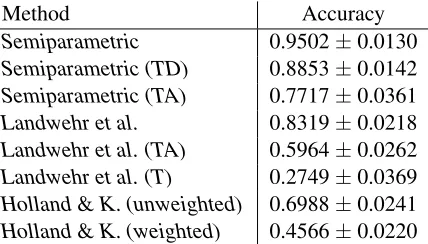
Method Accuracy
Semiparametric 0.9502±0.0130
Semiparametric (TD) 0.8853±0.0142
Semiparametric (TA) 0.7717±0.0361
Landwehr et al. 0.8319±0.0218
Landwehr et al. (TA) 0.5964±0.0262
Landwehr et al. (T) 0.2749±0.0369
Holland & K. (unweighted) 0.6988±0.0241
Holland & K. (weighted) 0.4566±0.0220
Table 1:Multiclass identification accuracy±standard error.
obtained from an EyeLink II system with a 500-Hz sampling rate (SR Research, Ongoode, Ontario, Canada) while reading sentences from thePotsdam Sentence Corpus(Kliegl et al., 2006). There are 144 sentences in the corpus, which we split into equally sized sets of training and test sentences. Individu-als read between 100 and 144 sentences, the training (testing) observations for one individual are the ob-servations on those sentences in the training (testing) set of sentences that the individual has read. Results are averaged over 10 random train-test splits. Each sentence is shown as a single line on the screen.
We study the semiparametric model discussed in Section 3 with MCMC inference as presented in Section 4 (denotedSemiparametric1). We employ a squared exponential covariance functionκ(x, x0) =
αexp−kx−2σx20k2
, where the multiplicative con-stant α is tuned on the training data by
cross-1An implementation is available at github.com/
abdelwahab/SemiparametricIdentification
validation and the bandwidth σ is set to the
av-erage distance between points in the training data.
The Beta and Dirichlet parameters λ and ρ are
set to one (Laplace smoothing), the prior p(η) for the Gamma parameters is uninformative. We use backoff-smoothing as discussed by Landwehr et al. (2014). We initialize the sampler with the maximum-likelihood Gamma fit and perform 10000 sampling iterations, 5000 of which are burn-in it-erations. As a baseline, we study the model by Landwehr et al. (2014) (Landwehr et al.) and sim-plified versions proposed by them that only use sac-cade type and amplitude (Landwehr et al. (TA)) or saccade type (Landwehr et al. (T)). We also study the weighted and unweighted version of the feature-based model of Holland & Komogortsev (2012) with a feature set adapted to the Potsdam Sentence Cor-pus data as described in Landwehr et al. (2014).
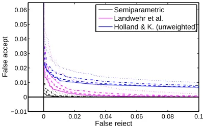
[image:7.612.77.291.264.386.2]move-0 0.02 0.04 0.06 0.08 0.1 −0.01
0 0.01 0.02 0.03 0.04 0.05 0.06
False reject
False accept
[image:8.612.325.524.57.181.2]Semiparametric Landwehr et al. Landwehr et al. (TA) Landwehr et al. (T) Holland & K. (unweighted) Holland & K. (weighted)
Figure 4:False-accept over false-reject rate when varyingτ.
ments to the 2D text structure, that is, to the way words are arranged into lines in a text. As in our empirical study each sentence is presented as a sin-gle line on screen, this 2D structure does not ex-ist. Moreover, Abdulin & Komogortsev (2015) only report accuracy improvements for their method in a setting where individuals have to be identified in the future based on data collected in the past (aging test), which is not the focus of our study.
We first study multiclass identification accuracy. All test observations of one particular individual constitute one test example; the task is to infer the individual that has generated these test observations. Multiclass identification accuracy is the fraction of cases in which the correct individual is identified. Table 1 shows multiclass identification accuracy for all methods, including variants of Semiparametric
discussed below. We observe that Semiparametric
outperformsLandwehr et al., reducing the error by more than a factor of three. Consistent with results reported in Landwehr et al. (2014), Holland & K.
(unweighted) is less accurate thanLandwehr et al.,
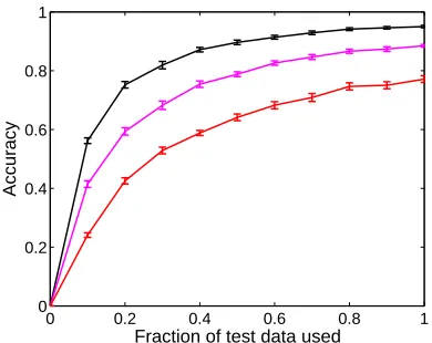
but more accurate than the simplified variants. We next study how the amount of data available at test time—that is, the amount of time we can observe a reader before having to make a decision—influences accuracy. Figure 3 (left) shows identification accu-racy as a function of the fraction of test data avail-able, obtained by randomly removing a fraction of sentences from the test set. We observe that iden-tification accuracy steadily improves with more test observations for all methods. Figure 3 (right) shows identification accuracy when varying the numberR
of individuals that need to be distinguished. We ran-domly draw a subset ofR individuals from the set
0 0.02 0.04 0.06 0.08 0.1
−0.01 0 0.01 0.02 0.03 0.04 0.05 0.06
False reject
False accept
Semiparametric Landwehr et al.
[image:8.612.84.284.57.180.2]Holland & K. (unweighted)
Figure 5: False-accept over false-reject rate when using 40% (dotted), 60% (dashed-dotted), 80% (dashed), and 100% (solid) of test observations, for selected subset of methods.
Method Area under curve
Semiparametric 0.0000119
Semiparametric (TD) 0.0000821
Semiparametric (TA) 0.0001833
Landwehr et al. 0.0001743
Landwehr et al. (TA) 0.0010371
Landwehr et al. (T) 0.0017040
Holland & K. (unweighted) 0.0027853
[image:8.612.315.536.239.362.2]Holland & K. (weighted) 0.0039978
Table 2:Area under the curve in binary classification setting.
of 251 individuals, and perform identification based on only these individuals. Results are averaged over 10 such random draws. As expected, accuracy im-proves if fewer individuals need to be distinguished. We next study a binary setting in which for each individual and each set of test observations a deci-sion has to be made whether or not the test observa-tions have been generated by that individual. This setting more closely matches typical use cases for the deployment of a biometric system. Let X¯ de-note the text being read at test time, and letS¯ de-note the observed eye movement sequences. Our model infers for each reader r ∈ R the marginal
likelihood p( ¯S|r,X¯,X,S(1:R)) of the eye
move-ment observations under the reader-specific model (Equation 3). The binary decision is made by dividing this marginal likelihood by the average marginal likelihood assigned to the observations by all reader-specific models, and comparing the result to a thresholdτ. Figure 4 shows the fraction of false accepts as a function of false rejects as the thresh-oldτ is varied, averaged over all individuals. The
0 0.2 0.4 0.6 0.8 1 0
0.2 0.4 0.6 0.8 1
Fraction of test data used
[image:9.612.89.284.55.210.2]Accuracy
Figure 6:Multiclass accuracy over number of test observations with standard errors forSemiparametricvariants.
reader-specific likelihood to novel test observations; we compute the same statistics again by normaliz-ing the likelihood and comparnormaliz-ing to a threshold τ.
Finally, Holland & K. (unweighted) and Holland
& K. (weighted) compute a similarity measure for
each combination of individual and set of test ob-servations, which we normalize and threshold
anal-ogously. We observe that Semiparametric
accom-plishes a false-reject rate of below 1% at virtually no false accepts;Landwehr et al. and variants tend to perform better than Holland & K. (unweighted)
and Holland & K. (weighted). Table 2 shows the
error under the curve for the experiment shown in Figure 4, as well as for variants of Semiparametric
discussed below.
We finally study the contribution of the individual model components for saccade type, saccade am-plitude, and fixation duration (see Figure 2) by re-moving the corresponding model components, as in
Landwehr et al. (2014). By Semiparametric (TD)
we denote a variant ofSemiparametricin which the variableatand the corresponding distribution is
re-moved, that is, only the distribution over the sac-cade type and duration is modeled.
Semiparamet-ric (TA) denotes a variant in which the variable
dt and the corresponding distribution is removed.
Figure 6 shows identification accuracy as a func-tion of the fracfunc-tion of test data available for model variants Semiparametric (TD) and Semiparametric (TA) in comparison toSemiparametric; results for these variants are also included in Table 1. Figure 7 shows the fraction of false accepts as a function of
0 0.02 0.04 0.06 0.08 0.1
−0.01 0 0.01 0.02 0.03 0.04 0.05 0.06
False reject
False accept
Semiparametric Full Semiparametric (TD) Semiparametric (TA)
Figure 7:False-accept over false-reject rate when varyingτfor theSemiparametricvariants.
false rejects in the binary classification setting dis-cussed above for these two model variants; Table 2 includes area under the curve results for the experi-ment shown in Figure 7. We observe that accuracy is substantially reduced when removing any model component. Note that if both the amplitude and du-ration components of the model are removed, it be-comes identical to the modelLandwehr et al. (T).
Training the joint model for all 251 individuals takes 46 hours on a single eight-core CPU (Intel Xeon E5520, 2.27GHz); predicting the most likely individual to have generated a set of 72 test sen-tences takes less than 2 seconds.
6 Conclusions
We have studied the problem of identifying read-ers unobtrusively during reading of arbitrary text. For fitting reader-specific distributions, we employ a Bayesian semiparametric approach that infers den-sities under a Gaussian process prior centered at the gamma family of distributions, striking a balance be-tween robustness to sparse data and modeling flex-ibility. In an empirical study with 251 individuals, the model was shown to reduce identification er-ror by more than a factor of three compared to ear-lier approaches to reader identification proposed by Landwehr et al. (2014) and Holland & Komogort-sev (2012).
Acknowledgements
[image:9.612.327.524.57.182.2]References
Evgeniy Abdulin and Oleg Komogortsev. 2015. Per-son verification via eye movement-driven text reading
model. InProceedings of the Sixth International
Con-ference on Biometrics: Theory, Applications and
Sys-tems.
Ryan P. Adams, Iain Murray, and David J.C. MaxKay.
2009. Gaussian process density sampler. In
Proceed-ings of the 21st Annual Conference on Neural
Infor-mation Processing Systems.
Roman Bednarik, Tomi Kinnunen, Andrei Mihaila, and Pasi Fr¨anti. 2005. Eye-movements as a biometric. In
Proceedings of the 14th Scandinavian Conference on
Image Analysis.
W. Robert Dixon. 1951. Studies in the psychology of reading. In W. S. Morse, P. A. Ballantine, and W. R.
Dixon, editors,Univ. of Michigan Monographs in
Ed-ucation No. 4. Univ. of Michigan Press.
Ralf Engbert, Antje Nuthmann, Eike M. Richter, and Reinhold Kliegl. 2005. SWIFT: A dynamical model
of saccade generation during reading. Psychological
Review, 112(4):777–813.
Tadayoshi Hara, Daichi Mochihashi, Yoshino Kano, and Akiko Aizawa. 2012. Predicting word fixations in text with a CRF model for capturing general reading
strate-gies among readers. InProceedings of the First
Work-shop on Eye-Tracking and Natural Language Process-ing.
Julian Heister, Kay-Michael W¨urzner, and Reinhold Kliegl. 2012. Analysing large datasets of eye move-ments during reading. In James S. Adelman, editor,
Visual word recognition. Vol. 2: Meaning and context,
individuals and development, pages 102–130.
Nils L. Hjort and Ingrid K. Glad. 1995. Nonparametric
density estimation with a parametric start. The Annals
of Statistics, 23(3):882–904.
Corey Holland and Oleg V. Komogortsev. 2012. Biomet-ric identification via eye movement scanpaths in
read-ing. In Proceedings of the 2011 International Joint
Conference on Biometrics.
Edmund B. Huey. 1908. The psychology and pedagogy
of reading. Cambridge, Mass.: MIT Press.
Pawel Kasprowski and Jozef Ober. 2004. Eye
move-ments in biometrics. InProceedings of the 2004
Inter-national Biometric Authentication Workshop.
Reinhold Kliegl, Antje Nuthmann, and Ralf Engbert. 2006. Tracking the mind during reading: The influ-ence of past, present, and future words on fixation
du-rations. Journal of Experimental Psychology:
Gen-eral, 135(1):12–35.
Oleg V. Komogortsev, Sampath Jayarathna, Cecilia R. Aragon, and Mechehoul Mahmoud. 2010. Biomet-ric identification via an oculomotor plant
mathemati-cal model. InProceedings of the 2010 Symposium on
Eye-Tracking Research & Applications.
Niels Landwehr, Sebastian Arzt, Tobias Scheffer, and Reinhold Kliegl. 2014. A model of individual
differ-ences in gaze control during reading. InProceedings
of the 2014 Conference on Empirical Methods on
Nat-ural Language Processing.
Peter J. Lenk. 2003. Bayesian semiparametric den-sity estimation and model verification using a
logistic-Gaussian process. Journal of Computational and
Graphical Statistics, 12(3):548–565.
Tom Leonard. 1978. Density estimation, stochastic
pro-cesses and prior information. Journal of the Royal
Sta-tistical Society, 40(2):113–146.
Franz Matties and Anders Søgaard. 2013. With blinkers on: robust prediction of eye movements across readers.
In Proceedings of the 2013 Conference on Empirical
Natural Language Processing.
Keith Rayner. 1998. Eye movements in reading and
in-formation processing: 20 years of research.
Psycho-logical Bulletin, 124(3):372–422.
Erik D. Reichle, Alexander Pollatsek, Donald L. Fisher, and Keith Rayner. 1998. Toward a model of eye
movement control in reading. Psychological Review,
105(1):125–157.
Ioannis Rigas, George Economou, and Spiros Fotopou-los. 2012a. Biometric identification based on the eye
movements and graph matching techniques. Pattern
Recognition Letters, 33(6).
Ioannis Rigas, George Economou, and Spiros Fotopou-los. 2012b. Human eye movements as a trait for
bio-metrical identification. InProceedings of the IEEE 5th
International Conference on Biometrics: Theory,
Ap-plications and Systems.
Ioannis Rigas, Oleg Komogortsev, and Reza Shadmehr. 2016. Biometric recognition via eye movements:
Sac-cadic vigor and acceleration cues. ACM Transaction
on Applied Perception, 13(2):1–21.
Surya T. Tokdar, Yu M. Zhuy, and Jayanta K. Ghoshz. 2010. Bayesian density regression with logistic
gaus-sian process and subspace projection. Bayesian
Anal-ysis, 5(2):319–344.
Ying Yang. 2009. Penalized semiparametric density
es-timation.Statistics and Computing, 19(1):355–366.
Youming Zhang and Martti Juhola. 2012. On biomet-ric verification of a user by means of eye movement
data mining. InProceedings of the 2nd International
Conference on Advances in Information Mining and