Abstract—The crystallization process consists in the
solid-liquid separation of organic and inorganic chemicals involving mass transfer of a solute dissolved in a liquid phase to a solid phase. The concentration zone widths let define the equilibrium or saturation line, metastable zone (first and second) and unstable or labile zone, and they are of prime importance for the design of optimal operation of cane sugar processes. This work has the goal to present a novel method to determine experimentally the concentration zone widths for commercial cane sugar (refined) using data and image acquisition approach. Crystal size distribution (CSD) analysis and micrograph sequences were used for determining the stability limits in terms of density. As a main result, we found that the width of the concentration zones (metastable and labile) increases nonlinearly whereas the saturation temperature (cooling) decreases in a range from 70 to 40 °C. The results are commented in terms of process operation conditions according to the required information by the cane sugar crystallization industry, in order to have an appropriate control of the supersaturation inside the process.
Index Terms—Cane sugar crystallization, concentration zone
widths, image and data acquisition, CSD.
I. INTRODUCTION
The crystallization process consists in the solid-liquid separation of organic and inorganic chemicals involving mass transfer of a solute dissolved in a liquid phase to a solid phase. At industrial conditions, the crystalline products require to have specific purity and crystal size distribution (CSD) instead of random distributions. The crystallization by cooling procedures is used when the solubility of the substance is an increasing function of the temperature. This operation is widely used in the industry for producing crystalline solids with a high purity at a cost relatively lower than other separation/purification operations [1]. In this form,
Manuscript received March 12, 2010. This work was supported in part by FOMIX CONACYT (National Council of Science and Technology) – Veracruz, Mex. under Project key: 37571.
E. Bolaños-Reynoso* is research-professor (PhD) with the Instituto Tecnologico de Orizaba. Oriente 9 No. 852. Col. E. Zapata. 94320 Orizaba, Ver. Mex. (corresponding author. Phone/fax: 52-272-725-70-56; e-mail: [email protected])
O. Velazquez-Camilo is CONACYT’s PhD. scholarship with Universidad Autonoma Metropolitana-Iztapalapa, 09340 Mexico, D.F. (e-mail: [email protected]).
L. Lopez-Zamora is research-professor (PhD) with the Instituto Tecnologico de Orizaba. 94320 Orizaba, Ver. Mex. (e-mail: llopezz02@ yahoo.com.mx).
J. Alvarez-Ramirez is research-professor (PhD) with the Universidad Autonoma Metropolitana-Iztapalapa, 09340 Mexico, D.F. (e-mail: [email protected]).
to obtain a specific CSD the supersaturation control plays an important role since it is a prerequisite for nucleation and growth. In turn, this is achieved through changes programmed in the cooling temperature, vacuum pressure, supersaturation, agitation rate and seeded crystal, among others [2]–[7]. One of the most important attributes in the crystallization processes is the presence of a continuous and a dispersed phase. By the effects of transport and physiochemical phenomena, the crystallization is realized through several steps, including nucleation, growth, occlusion and crystal attrition, leading to a distributed characterization of the physical and chemical properties of the product as the crystal size, forms, morphology, porosity, etc. [8], [9].
The operation of crystallizer should be oriented to meeting specified product quality measured as product purity and CSD [10]. In the literature, there are a lot of studies that apply the first-principle approach starting by mathematical models based on material, energy and population balances, with the aim of optimizing some variables of the process (CSD, crystal mass, density, etc.) to obtain better profit as much by the producer as by the client [11]-[13]. On the other hand, in the crystallization industry the direct design approach is based on the study of the metastable zones to the identification of an operation region allows to favor the crystal growth (seeded) and to avoid the spontaneous nucleación. Nevertheless, the study or application of the direct design approach has been less studied than the first-principle approach, because of the difficulty of disposing of laboratories with sophisticated equipments or due to the high cost of realizing experiments in plant. For the cane sugar, industrial process design and operation is still based on the usage of empirical concentration zone widths. To the best of our knowledge, a quantitative description of these concentration zone widths oriented for industrial applications is still lacking in the open scientific literature. Our aim is to present a novel method for determining the crystallization stability zones for industrial sugar cane using data and image acquisition. The approach uses both experimentation and modeling to obtain the saturation line and metastable and labile zone widths in terms of the solution density from measurements with a high-precision digital densimeter. We found that the width of the zones concentration increases nonlinearly as the saturation temperature decreases in a range from 70 to 40 °C.
Experimental Evaluation of the Concentration
Zone Widths in Cane Sugar Crystallization using
Data and Image Acquisition
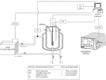
The experimental equipment was integrated by a data acquisition system (PCI-6025E, PCI-1407, SC-2345 and SCC-TC02 by National Instruments, Inc. (NI)), which was used to register the concentration (densimeter DMA-4500 by Anton-Paar) in a host computer and to control the temperature of the system by means of a programmable recirculation bath (Julabo F-34). The CSD was tracked in pseudo-line and registered by imaging acquisition system that included a monochrome camera (RS-170. Lens: 0.19 mm-pixel by NI) and microscope trinocular (48923-30 by Cole Palmer).
For the pseudoline measurement at every sampling time of the experimental runs and its particles analysis (crystals) through captured images, the software IMAQ Vision Builder (NI) was used. This image approach is an alternative in measuring both length and area of particles in a direct way through IMAQ Vision’s software. The technique consists of acquiring an image using a monochromatic camera with video RS-170 and 60 Hz crisscross (8 bits of resolution) and handling the light beam from a microscope trinocular. The camera captures an image square that is to be processed and cleaned. This avoids undesirable light variations. The latter is achieved through the threshold technique that allows obtaining only an image in gray scale. Interesting areas are isolated to be independently analyzed, and black pixels (crystals) are counted. The black pixels are compared with acceptation limits to decide if the object is present or not according to binary images (background) [14]. Then, a threshold technique approach, similar to that reported in further multiscale segmentation image approach, was used to compute the CSD features [15], [16].
The measurements and analysis of particles were carry out against a previous calibration through a Neubauer’s recount camera (simple calibration) in order to get a direct conversion from 1 pixel side to 200 μm (length). A pixel is defined as the smallest homogeneous unit in color that is part of the digital image. The pixels appear as small squares in white, black, or gray shades. In this work, a microscope with a 10x ocular lens with a 40x objective and an E square from Neubauer’s camera from 50 μm away, were used. This is equivalent to 20000 μm (10x40x50) per 100 pixels (length of pixel side). Thus, 1 μm is equal to 0.005 of the length of a pixel side [17]. There are different approaches for CSD measurements and
of the IMAQ Vision Builder system. Our software CSD Adq-Im receives the crystal length in micrometers from IMAQ system as input data. Then, CSD Adq-Im makes the relationship between the direct measurement D(1,0), considering our results as the microscopy approach, and the derivate measurement D(2,1) produced by LALLS. Later on, the derivative diameters D(3,2), D(4,3), and D(1,0) are calculated from each log-normal distribution of relative frequency from the LALLS approach. The latter approach (LALLS) obtains the derivative average diameter without necessarily requiring the particles total number from the slurry or solution at study. Finally, CSD Adq-Im carries out the calculations to obtain % number, % length, % surface, % volume, and others statistical properties from log-normal distributions of relative frequency [19]. The calculations were made following the mathematical formulism given by Marlven Instruments, Inc. [20] with its commercial equipment of particle analysis based on LALLS.
C.Obtaining of the Metastable and Labile Zone Widths To obtain the metastable and labile zones widths (MSZW), saturated solutions of commercial cane sugar (refined) at different equilibrium temperatures (40, 50, 60 and 70 °C) were prepared in a cooling batch crystallizer (Fig. 1). Here, the solution was cooling down in intervals of 1°C. For each temperature stationary state a solution sample in pseudoline was taken to measure the concentration (density) and the CSD. 3 ml of filtered solution was sampled (phase continues) with standard sugar paper (porosity of 19 µm) and 1 ml was introduced in the digital densimeter working to the atmospheric pressure. Then, to measure the CSD, 5 ml of solution without filtering was sampled and nuclei or crystals (smalls) images were acquired with the support of an imaging acquisition system.
The saturated solutions preparation was realized following a random design, being carried out four solutions with two replies, each one by different saturation temperatures. The established weight of each solution was 4500 g (g sugar/ml water), so that the sampling was not an importance variable to consider and to be able to handle the system as a solution constant volume. The proportions used to prepare the saturated solutions to its equilibrium temperature were obtained from Moncada’s equation [11].
2
0.0007 0.264 60.912
sat
Brix T T
Fig. 1 Cooling batch crystallizer.
Table 1. Electronics and instrumentation devices of a cooling batch crystallizer. Quantity Devices
1 6 L Glass crystallizer. Dimensions: 35 cm height and 14.4 cm internal diameter, 1.8 cm inferior dome height and 5 cm upper dome height., 2.55 L cooling - heating jacket
1
Generic motor of variable velocity with direct transmission from 0 rpm to 1,500 rpm, 60 Hertz, 127 VCA , agitation arrow of 14 inches (length) and diameter of ¼ inch, in stainless steel 316
1 Agitator/impeller of four rectangular ring with separation of 90° among each cross. Crosses’ longitude of 2 inches x 1inch of length for largeness in stainless steel 316. 2 Thermocouple J type. From 0 °C to 760 °C, wire-rope: 3 m.
1 Thermo-well in copper of 14 inches (length) and diameter of ½ inch.
1 Thermal isolation for high temperature with glass fiber of thickness ½ inch and recovered with paper aluminum foil.
1 Programmable recirculating bath (Julabo F-34), temperature range from -34 °C to 200 °C, pump flow of 15 Lpm, bath volume from 14 L to 20 L and 120 VCA/60 Hz.
1
Digital densimeter (Anton-Paar DMA-4500), measurement range from 0 g/cm3to 3 g/cm3,
feed sample to the cell: 1 ml of solution, measurement error in the temperature 0.1 °C and 1x10⁻⁵ g/cm3 in density. Measurement time for sample: usually 30 seconds. Interface
COM1, COM2 for connection RS-232 to computer.
1
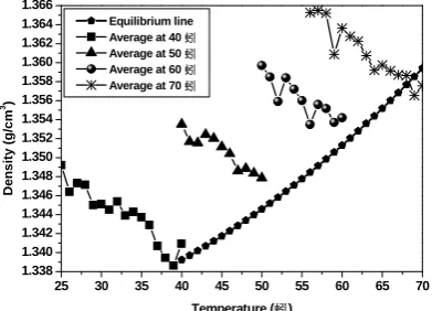
1.34093 to 1.34921 g/cm3, for 50 °C the temperature range of
cooling was from 50 to 40 °C and the concentration from 1.34785 to 1.35351 g/cm3, for 60 °C was from 60 to 50 °C
and the concentration from 1.3542 to 1.3597 g/cm3 and for 70
°C was from 70 to 53 °C and the concentration from 1.35769 to 1.36592 g/cm3. This concentration and temperature ranges
are the base to determine the concentration (critical points) of MSZW, complemented with CSD measurements and the acquired images, in order to quantify the CSD and to observe by means of micrographies the formation and growth of the crystal across the concentration zones.
Fig. 2 Average density in function of cooling down of 1 °C.
The saturation line (equilibrium) was obtained from (1) as a function of density:
5 6 2
sat 1.33 8.89 10 T 6.91 10 T
(2)
where sat is the saturation density in g/cm3 for each specific
equilibrium temperature. The density interval for a temperature range from 70 to 40 °C is from 1.3594073 to 1.3392435 g/cm3, respectively.
B.CSD and Micrographs Analysis
Fig. 3 shows the experimental data of the CSD in % volume with a log-normal distribution for each saturated solution (40, 50, 60 and 70 °C), being this the most representative with regard to the average of three experimental runs for every saturation temperature. The analysis of this figure is based on the quantification and observation of patterns on the crystal population for both cooling temperature and density range. In accordance with
[image:4.595.61.257.371.512.2]corresponds to the second metastable zone where the crystal growth dominates over the nucleation. When the cooling temperature decreases until to 32 °C, the % volume falls down drastically to 22 % in average and the average diameter D(4,3) decreases to about 82.3 µm. In turn, it is considered that this region represents the unstable or labile zone where the nucleation dominates over the crystal growth. Under these conditions, the CSD standard deviation is increased. This pattern can also be observed qualitatively by means of micrographic sequences in Fig. 4.
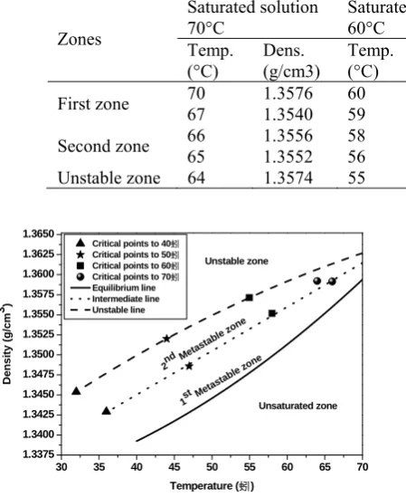
Fig. 3b to Fig. 3d illustrates the CSD for a solution saturated for 50, 60 and 70 °C, respectively. Table 2 resumes the CSD data from patterns (critical points of density) of three concentrations zones for each saturation temperature. C.Metastable and Labile Zone Widths
Fig. 5 shows the experimental density-temperature relationship where the critical points of MSZW are located by considering the minimum temperature for each temperature range presented in the Table 2. The density corresponding to every saturation temperature was located considering the Fig. 2 that presents the density averages of the experimental runs. From Fig. 5, we can observe that the zones width (metastable and labile) increases of non-linear form as the saturation temperature (cooling) decrease in a range from 70 to 40 °C. Meade and Chen [21] reported that the width for each zone for a cane sugar solution is constant and linear along the same cooling temperature range. However, our results showed that this is not the case, becoming a contribution for understanding of the saturation line, metastable zone and labile zone.
A non-linear second order regression was applied to the experimental data presented in the Fig. 5. The modeling equations describe the intermediate limit of the metastable zone and the limit of starting of the labile or unstable zone. Specifically, the intermediate line with R2= 0.998 is given by:
4 8 2
int ermediate 1.32 5.39 10 T 8.32 10 T
(3)
where intermediate is the density in the intermediate limit of the
metastable zone in g/cm3. The density interval of the model
by a temperature range from 70 to 40 °C is from 1.36148 to 1.34502 g/cm3, respectively. The labile line can be describing
according to the fitted equation with R2= 0.998: 25 30 35 40 45 50 55 60 65 70
1.338 1.340 1.342 1.344 1.346 1.348 1.350 1.352 1.354 1.356 1.358 1.360 1.362 1.364 1.366
Equilibrium line Average at 40 蚓
Average at 50 蚓
Average at 60 蚓
Average at 70 蚓
D
e
ns
it
y (
g/c
m
3)
Fig. 3 CSD of saturated solutions at: a) 40 °C, b) 50 °C, c) 60 °C and d) 70 °C.
Fig. 4. Micrographic sequence of growth crystals in saturated solution to 40°C. a) first metastable zone (40-37 °C), b) second metastable zone (36-33 °C) and c) labile zone (32 °C or smaller).
50 100 150 200 250 300 350 400 0 10 20 30 40 50 60 70 80 90 100 50 52 54 56 58 60 % V o lu m e Tem pera ture (蚓)
Size (
m) 100 200 300 400 500 600 0 10 20 30 40 50 60 70 80 90 100 54 56 5860 6264 6668 70 % V o lu m e Tem pera ture (蚓
)
Size (蚓
) d a b c 50 100 150 200 250 300 0 10 20 30 40 50 60 70 80 90 100 40 42 44 46 48 50 % V o lu m e Tem pera ture (蚓)
Size (
m) 50 100 150 200 250 300 0 10 20 30 40 50 60 70 80 90 100 24 26 2830 3234 3638 40 % V o lu m e Tem pera ture (蚓
)
Size (
[image:5.595.124.498.461.699.2]Fig. 5 Metastable and labile zone limits (MSZW) at the density – temperature diagram.
4 6 2
labile 1.32 8.32 10 T 3.7 10 T
(4)
Where labile is the density of starting limit of the labile zone
in g/cm3. The density interval of the model by a temperature
range from 70 to 40 °C is from 1.36269 to 1.34992 g/cm3,
respectively. Eqs. (3) and (4) shows clearly that the concentration limits are non-linear functions of temperature.
IV. CONCLUSION
The identification of the critical points of MSZW for commercial sugar cane was made in this work. A novel experimental method, based on cooling down sugar cane solutions and micrographs evaluation was used, yielding a close description of the concentration limits for the saturation line, the first and second metastable zone, and labile zone in density terms. In contrast to commercial practice, we found that the width of the zones increases in a non-linear form as the cooling saturation temperature decreases from 70 to 40 °C. The MSZW obtained experimentally should be useful for the design and operation of industrial crystallization equipment oriented to obtain specific products.
ACKNOWLEDGMENT
We thank Amira Antonio Acatzihua (CONACYT’s MS scholarship) for her collaborations in this paper.
REFERENCES
[1] Perry R. H. and D. Green W. Perry´s Chemical Engineers Handbook, 7a edition, McGraw-Hill. 2001.
[2] Quintana-Hernandez, P., Bolaños-Reynoso, E., Miranda-Castro, B. and Salcedo-Estrada, L. (2004). Mathematical Modeling and Kinetic Parameter Estimation in Batch Crystallization. AIChE Journal. 50 (7).
1407-1417.
[5] Srinivasakannan C., Vasanthakumar R., Iyappan K. and Rao, P. G. A. (2002). Study on crystallization of oxalic acid in batch cooling crystallizer. Chem. Biochem Eng. Q16 (3). 125-129.
[6] Mersmann, A. Crystallization Technology Handbook; Marcel Dekker: New York. 1995.
[7] Velazquez-Camilo, O., Alvarez-Ramirez, J. J. and Bolaños-Reynoso, E. (2009). Comparative Analysis of the Crystallizer Dynamics Type Continuous Stirred Tank: Isothermic and Cooling Case. Rev. Mex. Ing.
Quim. (RMIQ). 8 (1). 127-133.
[8] Salcedo-Estrada L. I., Quintana-Hernandez, P. A. and Bolaños-Reynoso E. (2002). Mathematical Modeling in Batch Crystallization. Chem. Eng. Assoc. Chem. Eng. Uruguay 3(21). 3-11.
[9] Christofides P. D., Shi D., El-Farra N. H., Li M. and Mhaskar P. (2006). Predictive control of particle size distribution in particulate processes.
Chemical Engineering Science. 61. 266-280.
[10] Rawlings J. B. and Miller S.M. (1994). Model identification and control strategies for batch cooling crystallizers. AIChe Journal. 40 (8).
1312-1327.
[11] Bolaños-Reynoso Eusebio, Xaca-Xaca Omar, Alvarez-Ramirez Jose, and Lopez-Zamora Leticia. (2008). Effect Analysis from Dynamic Regulation of Vacuum Pressure in an Adiabatic Batch Crystallizer Using Data and Image Acquisition. Ind. Eng. Chem. Res. 47 (23),
9426-9436.
[12] Fujiwara Mitsuko, Nagy Zoltan K., Chew Jie W. and Braatz Richard D. (2005). First-principles and direct design approaches for the control of pharmaceutical crystallization. Journal of Process Control. 15.
493-504.
[13] Zhou George X., Fujiwara Mitsuko, Woo Xing Yi, Rusli Effendi, Tung Hsien-Hsin, Starbuck Cindy, Davidson Omar, Ge Zhihong, and Braatz Richard D. (2006). Direct Design of Pharmaceutical Antisolvent Crystallization through Concentration Control. Crystal Growth & Design. 6 (4). 892-898.
[14] Hanks, J. Counting Particles of Cells using IMAQ Vision; Software is the Instruments, Application Note 107; National Instruments, Inc: Austin, TX, 1997.
[15] Wang, X. Z.; Calderon-De-Anda, J.; Roberts, K. J. (2007). Real-Time Measurement of the Growth Rates of Individual Crystal Facets using Imaging and Image Analysis. A Feasibility Study on Needle-Shaped Crystals of L-Glutamic Acid. Trans. IChemE, Part A, 85, 921–927. [16] Calderon-De-Anda, J.; Wang, X. Z.; Roberts, K. J. (2005). Multi-scale
Segmentation Image Analysis for the In-Process Monitoring of Particles Shape with Batch Crystallizers. Chem. Eng. Sci. 60, 1053–1065.
[17] Cordova-Pestaña, N. M.; Bolaños-Reynoso, E.; Quintana-Hernandez, P. A.; Briseño-Montiel, V. M. Developing of CSD Analysis Software from Electronic Microscopy Measurement; XXV AMIDIQ’s Memories: Mexico. 2004.
[18] Rawle, A. Basic Principles of Particle Size Analysis; Technical Paper Ref. WR141AT; Malvern Instruments: U.K., 1999.
[19] Quintana-Hernandez, P. A.; Moncada-Abaunza, D. A.; Bolaños-Reynoso, E.; Salcedo-Estrada, L. I. (2005). Evaluation of Sugar Crystal Growth and Determination of Surface Area Shape Factor. Rev. Mex. Ing. Quim. 4, 123–129.
[20] MasterSizer S Long Beb’s User Manual; Malvern Instruments. Ltd.: Westborough, MA, 1997.
[21] Meade, G. P. and Chen, J. C. Cane Sugar Handbook: A Manual for Cane Sugar Manufacturers and their Chemists. Wiley Publisher. 1977.
30 35 40 45 50 55 60 65 70
1.3375 1.3400 1.3425 1.3450 1.3475 1.3500 1.3525 1.3550 1.3575
1st M etasta
ble zo ne 2nd M
etasta ble zo
ne
Equilibrium line Intermediate line Unstable line
Densit
y
(g
/cm
3)
Temperature (蚓)
[image:6.595.56.281.65.340.2]