Efficient retrieval of tree translation examples for
Syntax-Based Machine Translation
Fabien Cromieres
Graduate School of Informatics Kyoto University
Kyoto, Japan
Sadao Kurohashi
Graduate School of Informatics Kyoto University
Kyoto, Japan
Abstract
We propose an algorithm allowing to effi-ciently retrieve example treelets in a parsed tree database in order to allow on-the-fly ex-traction of syntactic translation rules. We also propose improvements of this algorithm al-lowing several kinds of flexible matchings.
1 Introduction
The popular Example-Based (EBMT) and Statistical Machine Translation (SMT) paradigms make use of the translation examples provided by a parallel bilin-gual corpus to produce new translations. Most of these translation systems process the example data in a similar way: The parallel sentences are first word-aligned. Then, translation rules are extracted from these aligned sentences. Finally, the transla-tion rules are used in a decoding step to translate sentences. We use the term translation rule in a very broad sense here, as it may refer to substring pairs as in (Koehn et al., 2003), synchronous grammar rules as in (Chiang, 2007) or treelet pairs as in (Quirk et al., 2005; Nakazawa and Kurohashi, 2008).
As the size of bilingual corpus grow larger, the number of translation rules to be stored can easily become unmanageable. As a solution to this prob-lem in the context of phrase-based Machine Transla-tion, (Callison-Burch et al., 2005) proposed to pre-align the example corpora, but delay the rule extrac-tion to the decoding stage. They showed that using Suffix Arrays, it was possible to efficiently retrieve all sentences containing substrings of the sentence to be translated, and thus extract the needed trans-lation rules on-the-fly. (Lopez, 2007) proposed an
extension of this method for retrieving discontinu-ous substrings, making it suitable for systems such as (Chiang, 2007).
In this paper, we propose a method to apply the same idea to Syntax-Based SMT and EBMT (Quirk et al., 2005; Mi et al., 2008; Nakazawa and Kuro-hashi, 2008). Since Syntax-Based systems usually work with the parse trees of the source-side sen-tences, we will need to be able to retrieve effi-ciently examples trees from fragments (treelets) of the parse tree of the sentence we want to translate. We will also propose extensions of this method al-lowing more flexible matchings.
2 Overview of the method
2.1 Treelet retrieval
We first formalize the setting of this chapter by pro-viding some definitions.
Definition 2.1 (Treelets). A treelet is a connected subgraph of a tree. A treeletT1is asubtreeletof
an-other treeletT2 ifT1 is itself a connected subgraph
ofT2. We note|T|the number of nodes in a treelet.
If|T|= 1,Tis called anelementary treelet. A
lin-ear treelet is a treelet whose nodes have at most 1 child. A subtreerooted at node n of a treeT is a treelet containing all nodes descendants ofn.
Definition 2.2 (Sub- and Supertreelets). If T1 is a
subtreelet of T2 and |T1| = |T2| −1, we call T1
an immediate subtreelet ofT2. Reciprocally, T2 is
an (immediate) supertreelet of T1. Furthermore, if T2andT1are rooted at the same node in the original
tree, we say thatT2 is adescending supertreelet of T1. Otherwise it is anascending supertreeletofT1.
In treelet retrieval, we are given a certain treelet type and want to find all of the tokens of this type in the databaseDB. Each token of a given treelet type will be identified by a mapping from the node of the treelet type to the nodes of the treelet token in the database.
Definition 2.3 (Matching). Given a treelet T and a tree databaseDB, a matching ofTinDBis a func-tion M that associate the treelet T to a tree T in DB and every node of T to nodes ofT in such a way that: ∀n ∈ T, label(M(n)) = label(n) and
∀(n1, n2) ∈ T s.tn2 is a child of n1, M(n2) is a
child ofM(n1).
In the common case where the siblings of a tree are ordered, a matching must satisfy the additional restriction: ∀n1, n2 ∈ T, n1 <s n1 ⇔ M(n1) <s
M(n1), where <s is the partial order relation
be-tween nodes meaning “is a sibling and to the left of” We noteocc(T)(for “occurrences of T”) the set of all possible matchings fromT to DB. We will call computing T the task of finding occ(T). If
|occ(T)|= 0, we callTanempty treelet.Computing
a query treeTQmeans computing all of its treelets. Definition 2.4 (Notations). Although treelets are themselves trees, we will use the word treelet to emphasize they are a subpart of a bigger tree. We will noteT a treelet, andT a tree. TQis the query
tree we want to compute.DBwill refer to the set of trees in our database. We will use a bracket notation to describe trees or treelets. Thus “a(b c d(e))” is the tree at the bottom of figure 2.
2.2 General approach
There exists already a large body of research about tree pattern matching (Dubiner et al., 1994; Bruno et al., 2002). However, our problem is quite differ-ent from finding the tokens of a given treelet in a database. We actually want to find all the tokens of all of the treelets of a given query tree. The query tree itself is unlikely to appear in full even once in the database. In this respect, our approach will have many similarities with (Callison-Burch et al., 2005) and (Lopez, 2007), and can be seen as an extension of these works.
The basis of the method in (Lopez, 2007) is to look for the occurrences of continuous substrings us-ing a Suffix Array, and then intersect them to find the
occurrences of discontinuous substrings. We will have a similar approach with two variants. The first variant consists in using an adaptation of the con-cept of suffix arrays to trees, which we will call Path-To-Root Arrays (section 3.4), that allows us to find efficiently the set of occurrences of a linear treelet. Occurrences of non-linear treelets can then be com-puted by intersection. The second variant is to use an inverted index (section 3.5). Then the occurrences of all treelets, even the linear treelets, are computed by intersection.
The main additional difficulty in considering trees instead of strings is that while a string has a quadratic number of continuous substrings, a tree has in general an exponential number of treelets (eg. several trillion for the dependency tree of a 70 words sentence). There is also an exponential number of discontinuous substrings, but (Lopez, 2007) only consider substrings of bounded size, limiting this problem. We will not try to bound the size of treelets retrieved. It is therefore crucial to avoid computing the occurrences of treelets that have no occurrences in the database, and also to eliminate as much redun-dant calculation as is possible.
Lopez proposes to use Prefix Trees for avoiding any redundant or useless computation. We will use a similar idea but with an hypergraph that we will call “computation hypergraph” (section 3.2). This hypergraph will not only fit the same role as the Pre-fix Tree of (Lopez, 2007), but also will allow us to easily implement different search strategies for flex-ible search (section 6).
2.3 Representing positions
Whether we use a Path-to-Root Array or an inverted index, we will need a compact way to represent the position of a node in a tree. It is straightforward to define such a position for strings, but slightly less for trees. Especially, if we consider ordered trees, we will want to be able to compare the relative location of the nodes by comparing their positions.
the position of a node is a tuple consisting of its rank in a preorder (ie. children last) and a postorder (chil-dren first) depth-first traversal, and of its distance to the root. This allows to test easily whether a node is an ancestor of another, and their distance to each other. This allows in turn to compute by intersec-tion the occurrences of discontinuous treelets, much like what is done in (Lopez, 2007) for discontinuous strings. This is discussed in section 7.2.
3 Computing treelets incrementally
We describe here in more details how the treelets can be efficiently computed incrementally.
3.1 Dependence of treelet computation
Let us first define how it is possible to compute a treelet from two of its subtreelets. Let us consider a treelet T and two treelets T1 and T2 such that T =T1∪T2, where, in the equality and the union,
the treelet are seen as the set of their nodes. There are two possibilities. IfT1∩T2 =∅, then the root of T1 is a child of a node ofT2or vice-versa. We then
say thatT1andT2form a disjoint coverage
(abbrevi-ated as D-coverage) ofT. IfT1∩T26=∅, we will say
thatT1andT2form an overlapping coverage
(abbre-viated as O-coverage) ofT.
Given two treelets T1 and T2 forming a
cover-age ofT, we can computeocc(T)fromocc(T1)and occ(T2)by combining their matchings.
Definition 3.1 (compatibility for O-coverage). Let T be a treelet of TQ. Let T1 and T2 be 2 treelets
forming a O-coverage of T. Let M1 ∈ occ(T1)
and M2 ∈ occ(T2). M1 and M2 are
compat-ible if and only if M1|T1∩T2 = M2|T1∩T2 and
I(M1|T1\T2)∩ I(M2|T2\T1) =∅.
In the definition above,|Sis the restriction of a
func-tion to a setSandI is the image set of a function. If the children of a tree are ordered, we must add the additional restriction: ∀(n1, n2) ∈ (T1\T2)× (T2\T1), n1 <sn2⇔M1(n1)<sM2(n2).
Definition 3.2 (compatibility for D-coverage). Let T1 and T2 be 2 treelets forming a D-coverage
of T. Let’s suppose that the root n2 of T2 is a
child of node n1 of T1. Let M1 ∈ occ(T1) and M2 ∈ occ(T2). M1 andM2 are compatible if and
[image:3.612.363.503.45.149.2]only ifM2(n2)is a child ofM1(n1).
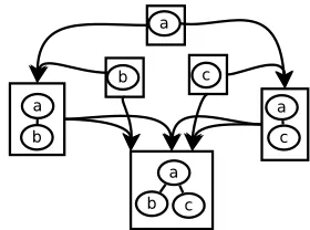
Figure 1: A computing hypergraph for “a(b c)”.
Definition 3.3 (intersection (⊗) operation). If two matchings are compatible, we can form their union, which is defined as (M1 ∪ M2)(n) = M1(n)
if n ∈ T1 and M2(n) else. We note occ(T1) ⊗ occ(T2) = {M1 ∪ M2 | M1 ∈ occ(T1), M2 ∈ occ(T2) and M1 is
compati-ble with M2 }. Then,we have the property: occ(T) =occ(T1)⊗occ(T2)
In practice, the intersection operation will be im-plemented using merge and binary merge algorithms (Baeza-Yates and Salinger, 2005), following (Lopez, 2007).
3.2 The computation hypergraph
We have seen that it is possible to computeocc(T)
from two subtreelets forming a coverage ofT. This can be represented by a hypergraph in which nodes are all the treelets of a given query tree, and every pair of overlapping or adjacent treelet is linked by an hyperedge to their union treelet. Whenever we have computed two starting points of an hyper-edge, we can compute its destination treelet. An example of a small computation hypergraph is described in figure 1.
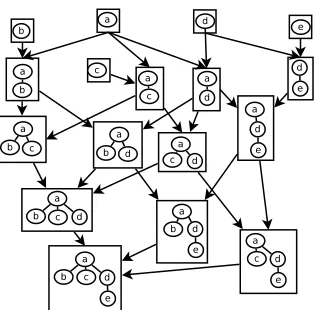
Figure 2: Inclusion DAG for the treea(bcd(e))
in (Lopez, 2007). Of course, the hypergraph is gen-erated on-the-fly during the traversal.
Furthermore, different traversals will define dif-ferent computation strategies, and we will be able to use some more advanced graph exploration methods in section 6.
3.3 The Immediate Inclusion DAG
In many cases (but not always: see section 4.3), the most optimal computation strategy should be to always compute a treelet from two of its imme-diate subtreelets. This is because the computation time will be proportional to the size of the small-est occurrence set of the two treelets, and thus the “cheapest” subtreelet is always one of the immedi-ate subtreelets. With this computation strimmedi-ategy, we can replace the general computation hypergraph by a DAG (Directed Acyclic Graph) in which every treelet point to its immediate supertreelets. An ex-ample is given on figure 2. We will call this DAG the (Immediate) Inclusion DAG.
Traversals of the Inclusion DAG should be pruned when an empty treelet is found, since all of its su-pertreelets will also be empty. The algorithm 1 pro-vide a general traversal of the DAG avoiding to com-pute as many empty treelets as possible. It uses a queueDof discovered treelets, and a data-structure C that associate a treelet to those of its subtreelets that have been already computed. Once a treeletT has been computed and is found to be non empty, we discover its immediate supertreeletsTS1,TS2, . . . (if they have not been discovered already) and addTto C(TS1),C(TS2), . . . . The operation min(C(T))
re-Algorithm 1: Generic DAG traversal
Add the set of precomputed treelets toD;
1
while∃T ∈ Ds.tT ∈precomputedor|C(T)|>2
2
do
popT fromD;
3
ifT in precomputedthen
4
occ(T)←precomputed[T];
5
else
6
T1,T2=min(C(T));
7
if|occ(T1)|= 0then
8
occ(T)← ∅;
9
else
10
occ(T)←occ(T1)⊗occ(T2);
11
forTS
∈supertree(T)do
12
ifocc(TS) =undefthen
13
AddTtoC(TS);
14
if|occ(T)|>0andTS / ∈ Dthen
15
AddTS to D;
16
trieve the 2 subtreelets fromC(T) that have the least occurrences. If one of them is empty, we can di-rectly conclude thatTis empty. No treelet whose all immediate subtreelets are empty is ever put in the discovered queue, which allows us to prune most of the empty treelets of the Inclusion DAG.
A treelet in the inclusion DAG can be computed as soon as two of its antecedents have been com-puted. To start the computation (or rather, “seed” it), it is necessary to know the occurrences of treelet of smaller size. In the following sections 3.4 and 3.5, we describe two methods for efficiently obtain-ing the set of occurrences of some initial treelets.
3.4 Path-to-Root Array
We present here a method to compute very effi-cientlyocc(T)whenTis linear. This method is sim-ilar to the use of Suffix Arrays (Manber and My-ers, 1990) to find the occurrences of continuous sub-strings in a text.
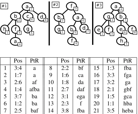
Definition 3.4 (Paths-to-Root Array). Given a la-beled tree T and a node n ∈ T, the path-to-root of n is the sequence of labels from n to the root. The Paths-to-Root Arrayof a set of treesDBis the lexicographically sorted list of the Path-to-Roots of every node inDB.
Pos PtR Pos PtR Pos PtR
1 3:4 a 8 2:2 bf 15 1:3 fba
2 1:7 a 9 1:6 ca 16 3:3 fga
3 2:6 af 10 1:8 da 17 3:2 ga
4 1:4 afba 11 2:7 daf 18 2:1 gbf
5 3:7 ba 12 3:1 ega 19 1:5 gca
6 1:2 ba 13 2:3 f 20 1:1 hba
[image:5.612.80.313.46.238.2]7 2:5 baf 14 3:8 fba 21 3:5 heba
Figure 3: Path To Root Array for a set of three trees. “Pos.” is the position of the starting point of a given path-to-root (noted as indexOfTree:positionInTree), and PtR is the sequence of labels on this root. The path-to-root are sorted in lexicographic order. We can find the set of occurrences of any linear treelet with a binary search. For example, the treelet a(b) corresponds to the label se-quence “ba”. With a binary search, we find that the path-to-root starting with “ba” are between indexes 5 and 7. The corresponding occurrences are then 3:7, 1:2 and 2:5.
memory to retrieve efficiently the pointed-to path-to-root. Once the Path-to-Root Array is built, for a linear treeletT, we can find its occurrences by a bi-nary search of the first and last path-to-root starting with the labels ofT. See figure 3 for an example.
Memory cost is quite manageable, since we only need 10 bytes per nodes in total. 5 bytes per pointer in the array (tree id: 4 bytes, start position: 1 byte), and 5 bytes per nodes to store the database in mem-ory (label id:4 bytes, parent position: 1 byte).
All the optimization tricks proposed in (Lopez, 2007) for Suffix Arrays can be used here, espe-cially the optimization proposed in (Zhang and Vo-gel, 2005).
3.5 Inverted Index and Precomputation
Instead of a Path-to-Root array, one can simply use an inverted index. The inverted index associates with every label the set of its occurrences, each oc-currences being represented by a tuple containing the index of the tree, the position of the label in the tree, and the position of the parent of the label in
the tree. Knowing the position of the parent will allow to compute treelets of size 2 by intersection (D-coverage). This is less effective than the Path-To-Root Array approach, but open the possibilities for the flexible search discussed in section 6.
Taking the idea further, we can actually con-sider the possibility of precomputing treelets of size greater than 1, especially if they appear frequently in the corpus.
4 Practical implementation of the traversal
4.1 Postorder traversal
The way we choose the treelet to be popped out on line 3 of algorithm 1 will define different computa-tion strategies. For concreteness, we describe now a more specific traversal. We will process treelets in an order depending on their root node. More pre-cisely, we consider the nodes of the query tree in the order given by a depth-first postorder traversal of the query tree. This way, when a treelet rooted at n is processed, all of the treelets rooted at a descendant ofnhave already been processed.
We can suppose that every processed treelet is as-signed an index that we note #T. This allows a con-venient recursive representation of treelets.
Definition 4.1 (Recursive representation). Let T be a treelet rooted at node n of TQ. We noteni the
ith child of n inT
Q. For all i, ti is the subtree of
T rooted at ni. We noteti = ∅ and#ti = 0 ifT
does not containni. The recursive representation of
Tis then:[n,(#t1,#t2, . . . ,#tm)]. We noteTithe
value#ti.
For example, ifTQ=“a(b c d(e))” and the treelets
“b” and “d(e)” have been assigned the indexes 2 and 4, the recursive representation of the treelet “a(b d(e))” would be [a,(2,0,4)].
Algorithm 2 describes this “postorder traversal”. DN ode is a priority queue containing the treelets
rooted atN odediscovered so far. The priority queue pop out the smallest treelets first. Line 14 maintain a listLof processed treelets and assign the index ofT in L to #T. Line 22 keeps track of the non-empty immediate supertreelets of every treelet through a dictionaryS. This is used in the procedure
Algorithm 2: DAG traversal by query-tree pos-torder
forNode in postorder-traversal(query-tree)do
1
Telem= [N ode,(0,0, ..,0)];
2
DN ode←Telem;
3
while|DN ode|>0do
4
T=pop-first(DN ode);
5
ifTin precomputedthen
6
occ(T)←precomputed[N ode.label];
7
else
8
T1, T2=min(C(t));
9
if|occ(T1)|= 0then
10
occ(T)← ∅;
11
else
12
occ(T)←occ(T1)⊗occ(T2);
13
AppendT toL;
14
#T ← |L|;
15
forTS in compute-supertree(T,#T)do
16
AddT toC(TS);
17
if|occ(T)|>0then
18
ifTS /
∈ DN odeand
19
root(TS)=Nodethen
AddTStoD;
20
for#tinC(T)do
21
Add#TtoS(#t);
22
descending supertreelets, and line 8 produces the as-cending supertreelet. Figure 4 describes the content of all these data structures for a simple run of the algorithm.
This postorder traversal has several advantages. A treelet is only processed once all of its immedi-ate supertreelets have been computed, which is op-timal to reduce the cost of the ⊗ operation. The way the procedure compute-supertreelets discover supertreelets from the info in S has also several benefit. One is that, by not adding empty treelets (line 18) to S, we naturally prevent the discovery of larger empty treelets. Similarly, in the next sec-tion, we will be able to prevent the discovery of non-maximal treelets by modifyingS. Modifications of
compute-supertreeletswill also allow different kind of retrieval in section 6.
4.2 Pruning non-maximal treelets
We now try to address another aspect of the over-whelming number of potential treelets in a query tree. As we said, in most practical cases, most of the larger treelets in a query tree will be empty. Still, it is
Algorithm 3: compute-supertrees
Input:T,#T
Output: lst: list of immediate supertreelets ofT m← |root(T)|;
1
foriin1. . . mdo
2
for #TSin
S(#Ti)do
3
ifroot(#TS)
6
=root(T)then
4
Tnew←[root(T), T0, ..#T0, . . . , Tm];
5
AppendTnewto lst;
6
Tnew←[parent(root(T)),(0, . . . ,#T, . . . ,0)];
7
AppendTnewto lst;
8
possible that some tree exactly identical to the query tree (or some tree having a very large treelet in com-mon with the query tree) do exist in the database. This case is obviously a best case for translation, but unfortunately could be a worst-case for our al-gorithm, as it means that all of the (possibly trillions of) treelets of the query tree will be computed.
To solve this issue, we try to consider a concept analogous to that of maximal substring, or substring class, found in Suffix Trees and Suffix Arrays (Ya-mamoto and Church, 2001). The idea is that in most cases where a query tree is “full” (that is all of its treelets are not empty), most of the larger treelets will share the same occurrences (in the database trees that are very similar to the query tree). We for-malize this as follow:
Definition 4.2 (domination and maximal treelets).
LetT1 be a subtreelet of T2. If for every matching M1 of occ(T1), there exist a matching M2 of occ(T2) such that M2|T1 = M1, we say that T1 is
dominated by T2. A treelet is maximal if it is not
dominated by any other treelet.
IfT1is dominated byT2, it means that all
occur-rences of T1 are actually part of an occurrence of T2. We will therefore be, in general, more interested
by the larger treeletT2 and can prune as many
non-maximal treelets as we want in the traversal. The key point is that the algorithm has to avoid discovering most non maximal treelets.The algorithm 2 can eas-ily be modified to do this. We will use the following property.
Property 4.1. GivenktreeletsT1. . . Tk withk
dis-tinct roots, all the roots being children of a same noden. We noten(T1. . . Tk)the treelet whose root
T d e b b(d)[Empty] b(e) b(d e)[Empty] c a a(b) a(b(e)) a(c) a(b c) a(b(e) c)
# 1 2 3 4 5 6 7 8 9 10 11 12 13
R d e b(..) b(1.) b(.2) b(1 2) c a(..) a(3.) a(5.) a(.7) a(3 7) a(5 7)
C - - - 1,3 2,3 4,5 - - 8,3 5,9 7,8 9,11 10,12
S - - 5 - - - - 9,11 10,12 13 12 13
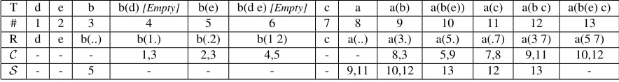
-Figure 4: A run of the algorithm 2, for the query tree a(b(d e) c). The row “T” represents the treelets in the order they are discovered. The row “#” is the index #T, and the row “R” is the recursive representation of the treelet. Also represented are the content ofCandSat the end of the computation. When a treelet is poped out ofDN ode, occ(T) is
computed from the treelets listed inC(T). If occ(T) is not empty, the entries of the immediate subtreelets of T inS
are updated with #T. We suppose here that|occ(b(d))|=0. Then, b(d e) is marked as empty and neither b(d) nor b(d e)
are added to the entries of their subtreelets inS. This way, when considering treelets rooted at the upper node “a”, the algorithm will not discover any of the treelets containing b(d).
children ofnareT1. . . Tk. Let us further suppose
that for alli, Ti is dominated by a descending
su-pertreelet Tid (with the possibility that Ti = Tid).
Then n(T1. . . Tk) is dominated by n(T1d. . . Tkd).
For example, if b(c) is dominated by b(c d), then a(b(c) e) will be dominated by a(b(c d) e).
In algorithm 2, after processing each node, we proceed to a cleaning of theSdictionary in the fol-lowing way: for every treelet T (considering the treelets by increasing size) that is dominated by one of its supertreelets TS ∈ S(T) and for every
subtreelet T0 of T such that T ∈ S(T0), we
re-placeT by TS in S(T0). The procedure
compute-supertreelets, when called during the processing of the parent node, will thus skip all of the treelets that are ”trivially” dominated according to property 4.1.
Let’s note that testing for the domination of a treeletTby one of its supertreletsTSis not a matter
of just testing if|occ(T)|=|occ(TS)|, as would be
the case with substring: a treelet can have less oc-currences than one of its supertreelets (eg. b(a) has more occurrences than b in b(a a) ). An efficient way is to first check that the two treelets occurs in the same number of sentences, then confirm this with a systematic check of the definition.
4.3 The case of constituent trees
We have focused our experiments on dependency trees, but the method can be applied to any tree. However, the computations strategies we have used might not be optimal for all kind of trees. In a de-pendency tree, nodes are labeled by words and most non-elementary treelets have a small number of oc-currences. In a constituent tree, many treelets con-taining only internal nodes have a high frequency
and will be expensive to compute.
If we have enough memory, we can solve this by precomputing the most common (and therefore ex-pensive) treelets.
However, it is usually not very interesting to re-trieve all the occurrences of treelets such as “NP(Det NN)” in the context of a MT system. Such very com-mon pattern are best treated by some pre-computed rules. What is interesting is the retrieval of lexical-ized rules. More precisely, we want to retrieve ef-ficiently treelets containing at least one leaf of the query tree. Therefore, an alternative computation strategy would only explore treelets containing at least one terminal node. We would thus compute successively “dog”, “NN(dog)” “NP(NN(dog))”, “NP(Det NN(dog))”, etc.
4.4 Complexity
Processing time will be mainly dependent on two factors: the number of treelets in a query tree that need to be computed, and the average time to com-pute a treelet.
LetNCbe the size of the corpus. It can be shown
quite easily that the time needed to compute a treelet with our method is proportional to its number of oc-currences, which is itself growing asO(NC).
[image:7.612.93.535.47.106.2]Database size (#nodes) 6M 60M Largest non-empty treelet size 4.6 8.7 Processing time (PtR Array) 0.02 s 0.7 s Processing time (Inv. Index) 0.02 s 0.9 s Size on disk 40 MB 500 MB
Figure 5: Performances averaged on 100 sentences.
grows approximately asO(m·NC0.5). It is also
pos-sible to bound the size of the retrieved treelets (only retrieving treelets with less than 10 nodes, for exam-ple), similarly to what is done in (Lopez, 2007). The number of treelets will then only grows asO(m).
The total processing time of a given query tree will therefore be on the order of O(m·N1.5
C ) (or
O(m·NC) if we bound the treelet size). The fact
that this give a complexity worse than linear with respect to the database size might seem a concern, but this is actually only because we are retrieving more and more different types of treelets. The cost of retrieving one treelet remain linear with respect to the size of the corpus. We empirically find that even for very large values ofNC, processing time remain
very reasonable (see next section).
It should be also noted that the constant hid-den in the big-O notation can be (almost) arbitrar-ily reduced by precomputing more and more of the most common (and more expensive) treelets (a time-memory trade-off).
5 Experiments
We conducted experiments on a large database of 2.9 million automatically parsed dependency trees, with a total of nearly 60 million nodes1. The largest
trees in the database have around 100 nodes. In or-der to see how performance scale with the size of the database, we also used a smaller subset of 230,000 trees containing near 6 million nodes.
We computed, using our algorithm, 100 randomly selected query trees having from 10 to 70 nodes, with an average of 27 nodes per tree. Table 5 shows the average performances per sentence. Con-sidering the huge size of the database, a
process-1This database was an aggregate of several Japanese-English
corpora, notably the Yomiuri newspaper corpus (Utiyama and Isahara, 2003) and the JST paper abstract corpus created at NICT(www.nict.go.jp) through (Utiyama and Isahara, 2007).
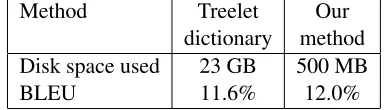
Method Treelet Our
dictionary method Disk space used 23 GB 500 MB
[image:8.612.83.319.48.116.2]BLEU 11.6% 12.0%
Figure 6: Comparison with a dictionary-based baseline (performances averaged over 100 sentences).
ing time below 1 second seems reasonable. The increase in processing time between the small and the large database is in line with the explanations of section 4.4. Path-to-Root Arrays are slightly bet-ter than Inverted indexes (we suspect a betbet-ter im-plementation could increase the difference further). Both methods use up about the same disk space: around 500MB. We also find that the approach of section 4.2 brings virtually no overhead and gives similar performances whether the query tree is in the database or not (effectively reducing the worst-case computation time from days to seconds).
We also conducted a small English-to-Japanese translation experiment with a simple translation sys-tem using Synchronous Tree Substitution Grammars (STSG) for translating dependency trees. The sys-tem we used is still in an experimental state and probably not quite at the state-of-the-art level yet. However, we considered it was good enough for our purpose, since we mainly want to test our algorithm is a practical way. As a baseline, from our cor-pus of 2.9 millions dependency trees, we automat-ically extracted STSG rules of size smaller than 6 and stored them in a database, considering that ex-tracting rules of larger sizes would lead to an un-manageable database size. We compared MT results using only the rules of size smaller than 6 to using all the rules computed on-the-fly after treelet retriev-ing by our method. These results are summarized on figure 6.
6 Flexible matching
that match by word or POS with the query tree.
6.1 Processing multi-Label trees
To do this, the inverted index will just need to include entries for both words and POS. For ex-ample, the dependency tree “likes,V:1 (Paul,N:0 Salmon,N:2 (and,CC:3 (Tuna,N:4)))” would pro-duce the following(node,parents) entries in the in-verted index: {N:[(0,1) (2,1) (4,3)], Paul:[(0,1)], Salmon:[(2,1)],. . .}. This allows to search for a treelet containing any combination of labels, like “likes(N Salmon(CC(N)))”.
We actually want to compute all of the treelets of a query treeTQlabeled by words and POS (meaning
each node can be matched by either word or POS). We can computeTQwithout redundant
computa-tions by slightly modifying the algorithm 2. First, we modify the recursive representation of a treelet so that it also includes the chosen label of its root node. Then, the only modifications needed in algo-rithm 2 are the following: 1- at initialization (line 3), the elementary treelets corresponding to every pos-sible labels are added to the discovered treelets set D; 2- in procedurecompute-supertrees, at line 8, we generate one ascending supertreelet per label.
6.2 Weighted search
While the previous method would allow us to com-pute as efficiently as possible all the treelets in-cluded in a multi-labeled query tree, there is still a problem: even avoiding redundant computations, the number of treelets to compute can be huge, since we are computing all combinations of labels. For each treelet of sizemwe would have had in a single label query tree, we now virtually have2mtreelets.
Therefore, it is not reasonable in general to try to compute all these treelets.
However, we are not really interested in comput-ing all possible treelets. In our case, the POS la-bels allow us to retrieve larger examples when none containing only words would be available. But we still prefer to find examples matched by words rather than by POS. We therefore need to tell the algorithm that some treelets are more important that some oth-ers. While we have used the Computation Hypertree representation to compute treelets efficiently, we can also use it to prioritize the treelets we want to com-pute. This is easily implemented by giving a weight
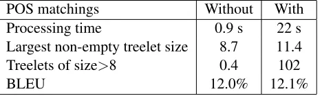
POS matchings Without With Processing time 0.9 s 22 s Largest non-empty treelet size 8.7 11.4 Treelets of size>8 0.4 102
[image:9.612.323.557.48.118.2]BLEU 12.0% 12.1%
Figure 7: Effect of POS-matching
to every treelet. We can then modify our traversal strategy of the Inclusion DAG to compute treelets having the biggest weights first: we just need to specify that the treelet popped out on line 3 is the treelet with the highest score (more generally, we could consider a A* search).
6.3 Experiments
Using the above ideas, we have made some experi-ments for computing query dependency trees labeled with both words and POS. We score the treelets by giving them a penalty of -1 for each POS they con-tain, and stop the search when all remaining treelets have a score lower than -2 (in other words, treelets are allowed at most 2 POS-matchings). We also re-quire POS-matched nodes to be non-adjacent.
We only have some small modifications to do to algorithm 2. In line 3 of algorithm 2, elementary treelets are assigned a weight of 0 or -1 depend-ing on whether their label is a word or POS. Line 5 is replaced by ”pop the first treelet with minimal weight and break the loop if the minimal weight is inferior to -2”. Incompute-supertreelets, we give a weight to the generated supertreelets by combining the weights of the child treelets.
Table 7 shows the increase in the size of the biggest non-empty treelets when allowing 2 nodes to be matched by POS. It also shows the impact on BLEU score of using these additional treelets for on-the-fly rule generation in our simple MT system. Im-provement on BLEU is limited, but it might be due to a very experimental handling of approximately matched treelet examples in our MT system.
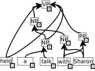
V-Figure 8: A packed forest.
mvt for verbs of movement instead of V).
7 Additional extensions
We briefly discuss here some additional extensions to our algorithm that we will not detail for lack of room and practical experiments.
7.1 Packed forest
Due to parsing ambiguities and automatic parsers errors, it is often useful to use multiple parses of a given sentence. These parses can be represented by a packed forest such as the one in figure 8. Our method allows the use of packed representation of both the query tree and the database.
For the inverted index, the only difference is that now, an occurrence of a label can have more than one parent. For example, the inverted in-dex of a database containing the packed forest of figure 8 would contain the following entries: {held: [(1,10a),(1,10b)], NP: [(6,9),(7,9),(9,10a)], VP:[(10,N)], PP:[(8,10b)], a:[(2,6)], talk:[(3,6)], with:[(4,7) (4,8)], Sharon:[(5,7) (5,8)]}. Where 10a and 10b are some kind of virtual position that help to specify thatheldandN P8 belong to the same
chil-dren list. We could also include a cost on edges in the inverted index, which would allow to prune matchings to unlikely parses.
The inverted index can now be used to search in the trees contained in a packed forest database with-out any modification. Modifications to the algorithm in order to handle a packed forest query are similar to the ones developed in section 6.
7.2 Discontinuous treelets
As we discussed in section 2.3, using a representa-tion for the posirepresenta-tion of every node similar to (Zhang
et al., 2001), it is possible to determine the distance and ancestor relationship of two nodes by just com-paring their positions. This opens the possibility of computing the occurrences of discontinuous treelets in much the same way as is done in (Lopez, 2007) for discontinuous substrings. We have not studied this aspect in depth yet, especially since we are not aware of any MT system making use of discontin-uous syntax tree examples. This is nevertheless an interesting future possibility.
8 Related work
As we previously mentioned, (Lopez, 2007) and (Callison-Burch et al., 2005) propose a method sim-ilar to ours for the string case.
We are not aware of previous proposals for ef-ficient on-the-fly retrieving of translation examples in the case of Syntax-Based Machine Translation. Among the works involving rule precomputation, (Zhang et al., 2009) describes a method for effi-ciently matching precomputed treelets rules. These rules are organized in a kind of prefix tree that al-lows efficient matching of packed forests. (Liu et al., 2006) also propose a greedy algorithm for matching TSC rules to a query tree.
9 Conclusion and future work
We have presented a method for efficiently retriev-ing examples of treelets contained in a query tree, thus allowing on-the-fly computation of translation rules for Syntax-Based systems. We did this by building on approaches previously proposed for the case of string examples, proposing an adaptation of the concept of Suffix Arrays to trees, and formaliz-ing computation as the traversal of an hypergraph. This hypergraph allows us to easily formalize dif-ferent computation strategy, and adapt the methods to flexible matchings. We still have a lot to do with respect to improving our implementation, exploring the different possibilities offered by this framework and proceeding to more experiments.
Acknowledgments
[image:10.612.115.272.46.163.2]References
R. Baeza-Yates and A. Salinger. 2005. Experimental analysis of a fast intersection algorithm for sorted se-quences. In String Processing and Information Re-trieval, page 1324.
N. Bruno, N. Koudas, and D. Srivastava. 2002. Holis-tic twig joins: optimal XML pattern matching. In
Proceedings of the 2002 ACM SIGMOD international conference on Management of data, page 310321. C. Callison-Burch, C. Bannard, and J. Schroeder. 2005.
Scaling phrase-based statistical machine translation to larger corpora and longer phrases. InProceedings of the 43rd Annual Meeting on Association for Compu-tational Linguistics, pages 255–262. Association for Computational Linguistics Morristown, NJ, USA. David Chiang. 2007. Hierarchical Phrase-Based
trans-lation. Computational Linguistics, 33(2):201–228, June.
M. Dubiner, Z. Galil, and E. Magen. 1994. Faster tree pattern matching. Journal of the ACM (JACM), 41(2):205213.
P. Koehn, F. J. Och, and D. Marcu. 2003. Statisti-cal phrase-based translation. InProceedings of HLT-NAACL, pages 48–54. Association for Computational Linguistics.
Z. Liu, H. Wang, and H. Wu. 2006. Example-based machine translation based on tree–string correspon-dence and statistical generation. Machine translation, 20(1):25–41.
A. Lopez. 2007. Hierarchical phrase-based translation with suffix arrays. InProc. of EMNLP-CoNLL, page 976985.
U. Manber and G. Myers. 1990. Suffix arrays: a new method for on-line string searches. In Proceed-ings of the first annual ACM-SIAM symposium on Dis-crete algorithms, pages 319–327, San Francisco, CA, USA. Society for Industrial and Applied Mathematics Philadelphia, PA, USA.
H. Mi, L. Huang, and Q. Liu. 2008. Forest based trans-lation.Proceedings of ACL-08: HLT, page 192199. Toshiaki Nakazawa and Sadao Kurohashi. 2008.
Syn-tactical EBMT system for NTCIR-7 patent translation task. InProceedings of NTCIR-7 Workshop Meeting, Tokyo, Japon.
C. Quirk, A. Menezes, and C. Cherry. 2005. De-pendency treelet translation: Syntactically informed phrasal SMT. In Proceedings of the 43rd Annual Meeting on Association for Computational Linguis-tics, page 279.
M. Utiyama and H. Isahara. 2003. Reliable measures for aligning japanese-english news articles and sentences. InProceedings of ACL, pages 72–79, Sapporo,Japon.
M. Utiyama and H. Isahara. 2007. A japanese-english patent parallel corpus. InMT summit XI, pages 475– 482.
M. Yamamoto and K. W. Church. 2001. Using suffix arrays to compute term frequency and document fre-quency for all substrings in a corpus. Computational Linguistics, 27(1):1–30.
Y. Zhang and S. Vogel. 2005. An efficient phrase-to-phrase alignment model for arbitrarily long phrase-to-phrase and large corpora. InProceedings of EAMT, pages 294– 301, Budapest, Hungary.
C. Zhang, J. Naughton, D. DeWitt, Q. Luo, and G. Lohman. 2001. On supporting containment queries in relational database management systems. In Pro-ceedings of the 2001 ACM SIGMOD international conference on Management of data, page 425436. H. Zhang, M. Zhang, H. Li, and Chew Lim Tan. 2009.