Abstract— Face recognition has assigned a special place to itself
because of its low intrusiveness, low cost and effort and acceptable accuracy. There are several methods for recognition and appearance based methods is one of the most popular one. Unfortunately most of the papers that have been published these years have just shown the results on the databases that are all without any noise and all of focus. But it is clear that for a real system all these problems can happen, so finding methods that are robust to such problems is important. In this paper we show that linear appearance based methods are robust to an acceptable degree to problems such as, when the camera is moving or it is defocus and when the image is influenced with Gaussian noise. For linear appearance based methods we chose Principal Component Analysis (PCA), Linear Discriminant Analysis (LDA) and Multiple Exemplar Discriminant Analysis (MEDA) that has shown better performance than other appearance based methods.
Index Terms— Linear Discriminant Analysis, Principal
Component Analysis, Multiple Exemplar Discriminant Analysis.
I. INTRODUCTION
Human identification recognition has attracted the scientists from so many years ago. Due to increasing in terrorism the needs for such systems have increased much more. The most important biometric systems which have been used during these years we can name fingerprint recognition, speech recognition, iris, retina, hand geometry and face recognition. For comparing biometric systems four features have been considered: intrusiveness, accuracy, cost and effort. The investigation has shown that among the other biometric systems, face recognition is the best one [1].
Among the various methods that has been applied to face recognition, appearance based methods have shown better
Manuscript received March 3, 2007.
M. Hajiarbabi, is an M.S. student in the Electrical and Computer Engineering Department, Isfahan University of Technology, Iran (corresponding author to provide phone: 09151107128; e-mail: m_arbabi@ ec.iut.ac.ir).
J. Askari, is with the Electrical and Computer Engineering Department, Isfahan University of Technology, Iran. (e-mail: [email protected]).
S. Sadri is with the Electrical and Computer Engineering Department, Isfahan University of Technology, Iran. (e-mail: [email protected]).
M. Saraee is with the Electrical and Computer Engineering Department, Isfahan University of Technology, Iran. (e-mail: [email protected]).
results, and have become the most popular method in face recognition. But a real system may encounter with some difficulties which are unexpected, for example when the camera or the subject is moving, when the camera is defocus or when the image has been influenced by noise, we need methods to be robust to such problems.
The goal of this paper is show the degree of robustness to camera moving, defocusing and noise immunity for linear appearance based methods.
The rest of the paper is organized as follows: in section 2 PCA, in section 3 LDA and in section 4 MEDA will be reviewed. In section 5 the RBF classifier and distance based classifier are reviewed. And finally in section 6 our work and the results are presented on the ORL [2] database.
II. PRINCIPAL COMPONANTANALYSIS
PCA is a method to efficiently represent a collection of sample points, reducing the dimensionality of the description by projecting the points onto the principal axes, where an orthonormal set of axes points in the direction of maximum covariance in the data. These vectors best account for the distribution of face images within the entire image space. PCA minimizes the mean squared projection error for a given number of dimensions, and provides a measure of importance (in terms of total projection error) for each axis.
Let us now describe the PCA algorithm [3]. Consider that Zi
is a two dimensional image with sizem×m. First we convert the matrix into a vector of sizem2. The training set of the n
face can be written as:
(
)
m nn Z Z Z
Z = 1, 2,..., ⊂ℜ 2× (1) Each of the face images belongs to one of the c classes. In face recognition the total images that belong to one person is considered as one class. For the training images the covariance matrix can be computed by:
(
)(
)
∑
=ΦΦ = − − =
Γ
n
i
T T
i
i Z Z Z
Z n 1
1 (2)
where
(
n)
m n× ℜ ⊂ Φ Φ Φ =
Φ 2
,..., , 2
1 and =
( )
∑
=n i Zi
n Z
1
1 is
the average of the training images in the database. As can be
The Evaluation of Camera Motion, Defocusing
and Noise Immunity for Linear Appearance
Based Methods in Face Recognition
easily seen the face images have been centered which means that the mean of the images is subtracted from each image. After computing covariance matrix, the eigenvectors and eigenvalues of the covariance matrix will be computed. Consider that U =
(
U U Ur)
⊂ℜm×r(
rpn)
2
,...,
, 2
1 be the
eigenvectors of the covariance matrix, only small parts of this eigenvectors, for exampler, that have the larger eigenvalues will be enough to reconstruct the image. So by having an initial set of face images Z ⊂ℜm2×n the feature vector corresponding to its related eigenface X ⊂ℜr×ncan be calculated by projecting Zin the eigenface space by
Z U
X = T (3)
III. LINEAR DISCRIMINANT ANALYSIS
LDA is used for projecting a set of training data. In face recognition and because of singularity problem it is common to use PCA first on the image and then apply LDA or MEDA to it. So consider that X =
(
X1,X2,...,Xn)
is a matrix containing thevectors in the training set. Xi is an vector that has been
calculated from an image after applying PCA to it. In LDA two matrixes within class scatter matrix and between class scatter matrixes is defined. This method finds an optimal subspace in which the between class scatter matrix to the within class scatter matrix will be maximized [4]. The between class scatter matrix is computed by
(
)(
i)
T ci i i
B n X X X X
S =
∑
− −=1
(4)
Where =
( )
∑
n=j Xj
n X
1
1 is the mean of the vectors in the training set and ⎟
∑
=⎠ ⎞ ⎜ ⎝ ⎛
= ni j i j i i X n X 1
1 is the mean of classi, and cis the number of the classes. The between class scatter matrix defines the average scattering of one class across the average of the total classes. The within class scatter matrix is computed by
∑ ∑
= ∈ ⎟ ⎠ ⎞ ⎜ ⎝ ⎛ − ⎟ ⎠ ⎞ ⎜ ⎝ ⎛ − = ci X n
T i i i i W i i X X X X S 1 (5)
The within class scatter matrix defines the data of one class across the average of the class. The optimal subspace is computed by
[
1, 2,..., 1]
max
arg = −
= c W T B T E
optimal c c c
E S E E S E E (6)
Where
[
c1,c2,...,cc−1]
is the set of eigenvectors of SBand SWcorresponding to c−1 greatest generalized eigenvalue λi and
1 ,..., 2 , 1 − = = S E i c E
SB i λi W i (7)
optimal
E is an optimal matrix which maximize the proportion of between class scatter matrix to the within class scatter matrix. This means that it maximize the scattering of the data that
belongs to different classes and minimize the scattering of the data belonging to the same class.
Thus the most discriminant answer for face vectors Xwould be [4]:
X E
P= optimalT ⋅ (8)
IV. MULTIPLEEXEMPLARDISCRIMINANTANALYSIS The problem of face recognition differs from other pattern recognition problems and so it needs different discriminant methods other than LDA. In LDA the classification of each class is based on just one sample and that’s the mean of each class. Because of lacking samples in face recognition problem it is better to use all the samples instead of the mean of each class for classification. Rather than minimizing the within class distance while maximizing the between class distance, multiple exemplar discriminant analysis (MEDA) finds the projection directions along which the within class exemplar distance (i.e. the distances between exemplars belonging to the same class) is minimized while the between-class exemplar distance (i.e. the distances between exemplars belonging to different classes) is maximized [5].
In MEDA the within class scatter matrix is computed by
(
)(
)
∑ ∑
∑
= = = − − = i i n j n k T i k i j i k i j C i iW X X X X
n S 1 1 1 2 1 (9) Where i
j
X is the jth image vector of ith class. By comparing it with the within class scatter matrix of LDA we see that in this method all the images in a class has participated in making the within class scatter matrix instead of using just the mean of the class as in LDA method. The between class scatter matrix is computed by
(
)(
)
∑∑
∑ ∑
= = = = ≠ − − = i j n k n l T j l i k j l i k C i C i j j j iB X X X X
n n S
1 1
1 1,
1
(10)
Contrary to LDA in which the means of each class and means of all samples made the between class scatter matrix, in MEDA all the samples in one class will be compared to all samples of the other class. The computation of Eoptimalis the
same as LDA.
V. CLASSIFIERS
For classification we used distance measures and also RBF neural network in order to compare their classification power. For distance measures we selected the following distances: Euclidean distance (L2):
( )
∑
(
)
= − = − = k i i i y x y x y x d 1 2 2 , (11) City block distance (L1):( )
2 1
1 1 ,
i i
k
i
i i i
z
z y x y
x d
λ
= − =
∑
=
(13)
Where λi is the eigenvalue of ith eigenvector.
RBF neural network is a powerful classification method for pattern recognition problems. It doesn't have the drawbacks of multi layer perceptron neural networks and trains much faster than it. Fig. 1 shows an RBF neural network.
[image:3.612.338.537.56.194.2]
Fig. 1: RBF neural network
Let P∈ℜr
be the input vector and C r
(
i u)
i∈ℜ 1≤ ≤ be the prototype of the input vectors. The output of each RBF units is as follows:2 2
exp ) (
i i i
C P P
R
σ − −
= (14)
Where σi is the width of the ith RBF unit. The jth output
( )
Pyj of an RBF neural network is
( )
( )
* ( ,)( )
,01
j w i j w P R p y
u
i i
i =
∑
+=
(15) WhereR0=1, w
( )
j,i is the weight of the ith receptive field to the jth output. The weights of first layer are all equal to one. The number of nodes in the second layer at first equals to the number of classes. Whenever two classes have intersection with each other a node is added to the second layer and a class is split into two subclasses. For further knowledge about RBF neural network the reader can refer to neural network references.VI. EVALUATIONOFCAMERAMOTION, DEFOCUSINGANDNOISEIMMUNITY
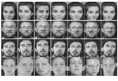
[image:3.612.54.298.178.298.2]In order to evaluate the algorithms mentioned above we used ORL database. ORL database contains 400 images that belong to 40 people with variety in scale and small variety in pose head. 5 images from every person was used as training set and the rest used as test set Fig. 2 shows a sample of this database.
Fig. 2: ORL database
We extracted 35 features for each method then by using RBF neural network and also Euclidean, City block and Mahalanobis distance we classified the data. As mentioned before, for LDA and MEDA we first applied PCA on the images and then applied LDA and MEDA on the new vectors in order to avoid the singularity problem. The input size of the neural network is equal to the size of the vector and the output size of it is 40 equal to number of classes.
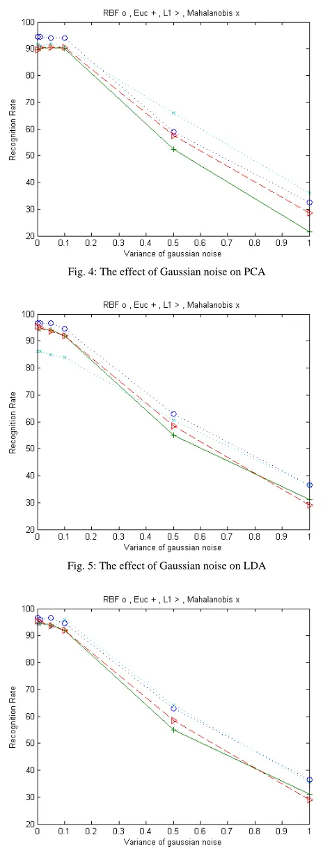
A. Noise immunity
For evaluation the effect of noise in recognition rate, we used Gaussian noise with zero mean and with variances 0.01, 0.05, 0.1, 0.5, and 1; we applied the noise just on the test images. Fig. 3 shows the testing images after applying the proposed noise to them; the first images from left have Gaussian noise with variance 0.01 and the right most images have Gaussian noise with variance1.
Fig. 3: Test images after applying Gaussian noise
[image:3.612.327.555.470.551.2]Fig. 4: The effect of Gaussian noise on PCA
Fig. 5: The effect of Gaussian noise on LDA
Fig. 6: The effect of Gaussian noise on MEDA
B. Camera motion immunity
For camera motion problem we shift the image to desired pixels with zero degree and then convolve it with the origin picture and so the camera motion is simulated. Fig. 7 shows the
images from left to right after applying the filter with 4, 8, 16, 24 and 40 pixels shifting and convolving with the original image.
Fig. 7: Test images after applying camera motion
[image:4.612.324.554.98.179.2]Fig. 8-10 shows the recognition rate for PCA, LDA and MEDA respectively. The results show good immunity in the case of camera motion. Something which is quite interesting in the results is the increasing in recognition rate, although we are increasing the camera motion. The reason can be this: applying some changes to the images, cause the features vectors extracted from the images and that belong to the same class becomes closer to each other in the subspace, so it increases the recognition rate although everyone expect it to decrease. Another thing which is interesting is the RBF neural network behavior. At first and when there is no or little camera motion it quite outperforms other classifiers, but as the camera motion increases the performance of RBF decreases more rapidly than other classifiers.
[image:4.612.328.546.383.568.2]Fig. 9: The effect of camera motion on LDA
Fig. 10.: The effect of camera motion on MEDA
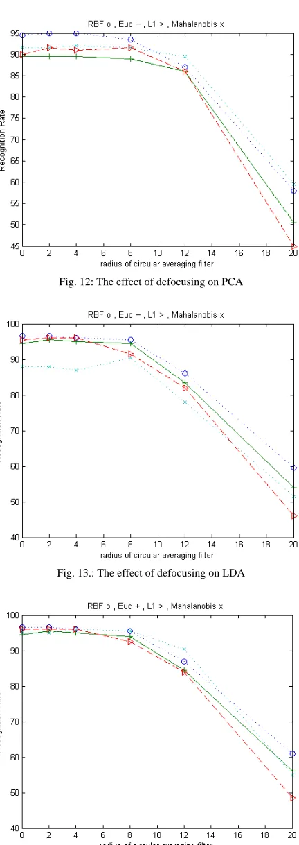
C. Defocusing immunity
[image:5.612.55.283.53.455.2]For defocusing we used a circular average filter with radius 2, 4, 8, 12 and 20, which was convolved with the origin image. Fig. 11 show the images from left to right after convolving the filters with radius 2, 4, 8, 12 and 20 with them respectively.
Fig. 11: Test images after applying defocusing
Fig. 12-14 show the recognition rate for PCA, LDA and MEDA respectively. The results show good immunity in the case of defocusing. The results show even when the recognizing of the test images is difficult for human eye, it have been recognized by the appearance based methods.
Fig. 12: The effect of defocusing on PCA
Fig. 13.: The effect of defocusing on LDA
[image:5.612.50.281.567.654.2]VII. CONCLUSION
In this paper we showed that the linear appearance based methods are immune to noise, defocusing and camera motion to acceptable degree. This work can be applied to other methods to see their results on such problems.
REFERENCES
[1] R. Hietmeyer, “Biometric identification promises fast and secure processing of airline passengers,” The Int’l Civil Aviation Organization Journal, vol. 55, no. 9, 2000, pp. 10–11.
[2] ORL database: http://www.camorl.co.uk.
[3] M. Turk, and A. Pentland,, “Eigenfaces for recognition,” J. Cognitiv Neurosci., vol. 3, 1991, pp. 71–86.
[4] K. Fukunaga,, Introduction to statistical pattern recognition, 2nd ed. San
Diego, CA: Academic Press, 1990, pp. 445-450.
[5] Sh. K. Zhou, and R.Chellappa, “Multiple-exemplar discriminant analysis for face recognition” Center for Automation Research and Department of Electrical and Computer Engineering University of Maryland,