Abstract—The homogeneous equilibrium model improved (HEMI) is for determining the mass flux of all fluids in piping systems. Existing homogeneous equilibrium models tend to underpredict overall pressure drops in piping systems as the flow length is increased. HEMI has corrected the fundamental defect and the associated flow equation is both mathematically and physically satisfactory. The HEMI can also be extended to account for non-equilibrium effects. The resulting calculation sets are compared with experimental data.
Index Terms— Homogeneous equilibrium model improved, nonequilibrium effects, pipe flows, pressure relief system.
I. INTRODUCTION
This article presents an improved homogeneous equilibrium model for estimating the mass flux of all fluids in piping systems. Piping systems mean fluids flow in pipes, tubes or ducts at a constant diameter or changing diameters, elevations, and directions. Determining accurate flow capacities and pressure drops in piping systems is important in designing pressure relief systems. The goal of pressure relief systems is to prevent excessive pressure accumulation in a pressure vessel for all credible emergency scenarios. An improperly designed relief system may result in catastrophic failures. Therefore the pressure relief system should be sized with as much certainty as possible for proper protection of the pressure vessel or system. Currently, a homogeneous equilibrium model (HEM) is used extensively in designing the pressure relief system because it gives conservative results (smallest flow capacity). However, the existing homogeneous equilibrium model tends to underpredict overall pressure drops in piping systems as the flow length is increased. The homogeneous equilibrium model improved (HEMI) has corrected the fundamental defect which caused this underprediction.
HEMI requires an accurate correlation of pressure–specific volume. This greatly enhances calculation capabilities when handling compressible fluids in piping systems. The correlation of pressure-specific volume can be obtained by flash calculations. The flow path can be either isenthalpic or isentropic. For two-phase flow, the difference between isenthalpic and isentropic is not significant. HEMI provides accurate and conservative results because the associated flow equation is mathematically and physically
Manuscript received June 25, 2010.
J. S. Kim and H. J. Dunsheath are with Bayer Business and Technology Services, Baytown, TX 77523 USA ( e-mail: jung.kim@bayertechnology .com; [email protected]).
.
satisfactory. Additionally, HEMI can be extended to account for nonequilibrium effects for flashing flow. The resulting calculation sets are compared with experimental data.
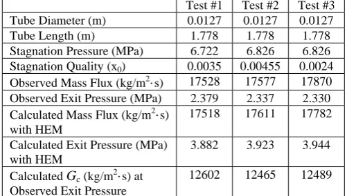
II. UNCERTAINTIES OF EXISTING PIPE FLOW MODELS Sozzi and Sutherland [1] performed extensive tests for high pressure saturated and subcooled water. The test data for low stagnation quality (0.001 < x0 < 0.005, mass fraction of vapor in two-phase) saturated water on Nozzle 2 are of particular interest. Nozzle 2 had a well-rounded entrance (no entrance loss). The test data shown in Table I (selected out of 25 tests in Table V) are for a 1.778 m straight horizontal long run of 12.7 mm diameter tubing. Isenthalpic flash calculations were performed to generate correlations of pressure-specific volume. This is to ensure that the calculation results would be conservative since the isenthalpic flow path yields a lower bound estimate of mass flux. The existing HEM results are obtained using a computer program called CCflow, a flow capacity calculation program for use with the CCPS Guidelines book “Pressure Relief and Effluent Handling Systems” [2]. AIChE Design Institute for Emergency Relief Systems (DIERS) recommends the use of the homogeneous equilibrium model in the pressure relief system calculations.
The experimental data in Table I show that the existing homogenous equilibrium model predicts less conservative mass flux results than expected. In addition, the calculated exit pressures deviate significantly from the observed ones. One could easily calculate the critical or choked mass flux Gc using equation (3) if the exit pressure is known. The difference between the observed mass flux and the calculated critical mass flux at observed exit pressure is, as expected, significant. Generally nonequilibrium results in appreciable mass flux increase. The calculated mass flux values at observed exit pressures support the nonequilibrium hypothesis. Consequently, it is obvious that the significant difference in exit pressures is an indication of nonequilibrium.
A Homogeneous Equilibrium Model Improved
for Pipe Flows
[image:1.595.301.552.660.802.2]Jung Seob Kim and Heather Jean Dunsheath
Table I
Sozzi and Sutherland Nozzle 2 Test Data vs. HEM Predictions Test #1 Test #2 Test #3
Tube Diameter (m) 0.0127 0.0127 0.0127
Tube Length (m) 1.778 1.778 1.778
Stagnation Pressure (MPa) 6.722 6.826 6.826
Stagnation Quality (x0) 0.0035 0.00455 0.0024
Observed Mass Flux (kg/m2·s) 17528 17577 17870 Observed Exit Pressure (MPa) 2.379 2.337 2.330 Calculated Mass Flux (kg/m2·s)
with HEM
17518 17611 17782
Calculated Exit Pressure (MPa) with HEM
3.882 3.923 3.944
The HEM results in Table I were also in good with the observed values. Therefore, the mass flux of the HEM was definitely overpredicted since equilibrium conditions gave more conservative results.
III. HOMOGENEOUS EQUILIBRIUM MODEL
HEM uses the following pipe flow equation for horizontal pipe flows [3], [4]:
2 0
2 0
0 2 2
ln 2
) 1 ( ln
2 ) 1 ( ln 2
) 1 (
N P N
dP
v v N
v dP
G avg
where G is the mass flux in pipe flows, is the density of the fluid, P is the pressure in pipe flow systems, N is the overall loss coefficient, and
v
is the specific volume of the fluid.
dP,arithmeticavgP, is satisfactory mathematically, but not physically since actual average density is computed for n data points of density over a constant interval of pressure as the following:
n
i i avg
actual
n 1
1 1
1
The HEM provides only a mathematical solution. This means that the HEM does not represent the true compressible flow behavior in piping systems. The arithmetic average density should not be used in the pipe flow equation for compressible flow. But
dP can easily be seen in textbooks for flow equations for compressible flows. Using the arithmetic average density in the pipe flow equation signals overprediction in mass flux. Therefore, the HEM significantly underpredicts overall pressure drop in the piping system for two-phase flow as shown in Table I. The underprediction in overall pressure drop increases with increasing flow lengths (overall loss coefficient). Also if the back pressure of a pressure relief valve is also to be determined for a given rated capacity of the pressure relief valve, then the homogeneous equilibrium method will underestimate the back pressure. Pressure relief valves are the most commonly used relief device. The pressure relief valve performance and stability are affected by the back pressure. Therefore, a mandatory requirement of ASME - Pressure Vessel Code [5]is that the outlet piping of the relief valve be such that the developed back pressure will not reduce the relieving capacity below the flow required to protect the equipment.IV. HOMOGENEOUS EQUILIBRIUM MODEL IMPROVED On the other hand, HEMI uses the following pipe flow equation for horizontal pipe flows:
2
2 2
avg v N vdv
vdP G
(1)
vdP
P vavg
1 (2)
dv dP
Gc2 (3)
G2 – Gc2= ~ 0 at choked conditions (4)
The pipe flow equation (1) is derived from the Bernoulli equation with proper manipulation not to include
dP. HEMI predicts accurate and conservative estimates of homogeneous equilibrium flow conditions because
vdP ,v
arithmeticavg P , is both mathematically and physically satisfactory. The actual average specific volume is computed for n data points of specific volume over a constant interval of pressure as the following:
n i
i avg v
n v
1
1
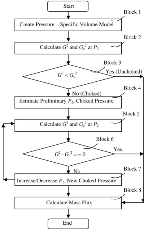
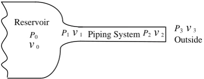
To illustrate the improved homogenous equilibrium model, the calculation procedure shown in Fig. 1 will be explained in detail below. Fig. 2 is a typical configuration of a pressure relief piping system. The pressure relief piping system often includes a rupture disk. A rupture disk is a non-reclosing pressure relief device actuated by the inlet static pressure.
Calculate G2 and Gc 2
at P3
G2 < Gc2
Calculate G2 and Gc 2
at P2
G2 - Gc2 = ~ 0
End
Block 1
Block 2
Block 5 Block 4 Block 3
Block 8 Block 6
Block 7 No (Choked)
Yes
No
Create Pressure – Specific Volume Model
Increase/Decrease P2, New Choked Pressure
Calculate Mass Flux
Estimate Preliminary P2, Choked Pressure
[image:2.595.306.539.383.754.2]Yes (Unchoked) Start
The flow is from a large upstream reservoir 0 (named station 0), through a constant-area run of pipe entrance 1 (named station 1). The flow from the pipe entrance discharges to the outside 3 (named station 3) of the end of the pipe 2 (named station 2).
Fig. 1 is a procedure block diagram for the mass flux and exit pressure calculations. The first step, block 1, is to create pressure-specific volume models using data obtained by flash calculations on either an isentropic or isenthalpic flow path. A pressure-specific volume model with two constants, and
, by Simpson [4]as the following fits the data for a broad range of fluids, and is suitable for integration:
1 1
2 1
1 2
P P v
v (5)
Estimating accurate specific volume is extremely important in calculating the mass flux in piping systems. Single phase or two-phase flow requires at least one P-v correlation while at least two P-v correlations in series are recommended for subcooled liquid. For subcooled liquid, the first P-v model can be based on two data points. The second data point is at the saturated pressure. The pressure-specific volume model “constant” for the two data points is 1.0. A general guideline for selecting data points is presented as the following:
The second step, block 2, is to calculate G2 and Gc2 at outside pressure (P2 = P3). All calculations are often based on two segments: a frictionless section from P0 to P1 and a friction section from P1 to P2 as shown in Figure 2. More segments can be considered if necessary. Although the pressure range from P1 to P2 is more desirable for
v
avg in flow equation (1), thev
avgcan be calculated for a pressure range from P0 to P2. This does not give significant differences for a large N(overall loss coefficient) piping system. The pressure value of P1 can be obtained by solving the following equation:
2
2 2
2 0 1
0
avg p p p
p
v N vdv
vdp
vdv vdp G
(6)For most pressure relief piping systems, the pipe length L, the inside pipe diameter D, and the total frictional loss coefficient
K are known. An overall loss coefficient N is calculated as the following:
K D
L f
N4 (7)
A Fanning friction factor of f can be taken for fully turbulent flow. More rigorous calculation methods for the friction factor can be considered if the overall loss coefficient is sensitive to the friction factor. For such a case, a simple polynomial equation for fluid viscosities varying with pressure can be developed in the same manner as the P-v model. G2 is estimated by solving flow equation (1) by either direct integration, numerical integration, analytical integration, or a simple way using direct data points. Gc2 is estimated using equation (3) by taking the pressure derivative with respect to the specific volume at P3. Gc2 can also be estimated at a small pressure increment dP as well as the corresponding specific volume change at the small pressure increment.
The third step, block 3, is to determine if the piping system is choked at station 3 pressure. If the estimated G2 is greater than the estimated Gc2, it means the system is choked. Thus, it is required to proceed with the next step. If not, the mass flux is calculated at block 8. Incompressible fluid is generally not choked. Thereafter, a preliminary choked pressure is estimated, block 4. A good initial choked pressure ensures fast convergence. The choked pressure can be determined by the point of intersection between curves G2 and Gc2. The point of intersection indicates choked conditions. Or simply take around 50% of P0 as the initial choked pressure estimate. For the accurate choked pressure, equation (4) is solved by trial and error by changing P2 until G2-Gc2 = ~0 (within error tolerance), blocks 5 - 7. New P2 (choked pressure) is (G2-Gc2) (Previous P2) / [(2.0)(G2)] + Previous P2. Factor 2, which is adjustable, is to achieve stable convergence. The Newton-Raphson Method can also be used as an alternative for the partial substitution method.
The final step, block 8, is to determine the homogeneous equilibrium mass flux along with unit conversion as the following:
G = [G2(106)]0.5
However, experimental data show that significant nonequilibrium exists for two-phase flow. The nonequilibrium is generally believed to be mostly from thermal nonequilibrium. HEMI can be extended to account for the nonequilibrium effects. The authors are proposing the following preliminary nonequilibrium factor until complete comprehensive correlations are available.
The overall pressure drops in piping systems consist of the following three pressure drop terms:
2
0 P
P Ptotal
(8) v
G Pkinetic
2
2 1
[image:3.595.51.256.143.222.2] (9)
Fig. 2. Typical configuration of a pressure relief piping system. i
P3
v
3Outside
P2
v
2P1
v
1
P0
v
0Reservoir
Piping System
Table II
Data Point Guidelines for Pressure-Specific Volume Correlations One P-
v
model P0 , (P0 +P3)/2 , P3Two P-
v
modelsavg friction G v
N
P 2
2
(10) friction
kinetic total
ansion P P P
P
exp (11)
Out of the three pressure loss terms, the pressure drop for expansion contributes the most to the nonequilibrium effects in the piping systems. The nonequilibrium factor (NF) can be defined as the following:
NF = (1+Pexpansion / Ptotal)0.5 (12) Thus, the nonequilibrium mass flux (NEMF) and the exit pressure (NEEP) are calculated as the following:
NEMF = (Equilibrium Mass Flux) (NF) (13) NEEP = P0 - (Ptotal)(NF)2.3 (14) The actual pressure drop for nonequlibrium two-phase flow is likely to be greater than the pressure drop which is generally proportional to the square of NF. However, equations (12) and (14) are temporary and valid for the specific test conditions (0.001 < x0 < 0.005 and N=2.61).
V. EXAMPLE USING HEMI
The following example uses a simplified calculation approach for Test #1 in order to make the calculation procedure easier to follow. The fluid is saturated water with stagnation quality of 0.0035 at 6.722 MPa in a pressure vessel. The following three data points are prepared based on an isenthalpic flow path.
Using the three data points and equation (5), the following two simultaneous equations are obtained:
1 1
2 1 1 2 P P v v
1 1
3 1 1 3 P P v v
A simple bisection routine could solve for and The results are:
= 3.509350 = 1.255901
Therefore, the specific volume at any pressure point can be obtained easily with the following pressure-specific volume model:
v
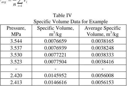
= 0.0014378 [3.509350((6.722/P)1.255901 -1) +1]The following specific volume data are prepared using the pressure-specific volume model above. Average specific volume is computed for n data points of specific volume over a constant interval of 6.8947 Pa (1 psi) as the following:
n i i avg v n v 1 1It is assumed that the overall loss coefficient in the piping system is independent of the Reynolds number and the tube absolute roughness is 0.01016 mm. The value of the absolute roughness of the test tube was not available. Darby et al. [3] also used absolute roughness of 0.01016 mm for the test tube. Based on the tube length of 1.778 m and the typical Fanning friction factor of 0.00466, the overall loss coefficient of 2.61 is calculated as the following:
61 . 2 0 0127 . 0 778 . 1 ) 00466 . 0 ( 4
4
K
D L f N
First, it is required to check if the piping system is choked at 2.413 MPa assumed as P3 pressure (tube outside).
8 . 162 2 ) 0056153 . 0 ( 61 . 2 2 0146616 . 0 ) 722 . 6 413 . 2 ( 0056153 . 0 2 2 2 2 2 avg avg v N vdv P v G 4 . 105 ) 0146616 . 0 0145952 . 0 ( ) 413 . 2 420 . 2 ( 2 dv dP Gc
Since G2 is greater than Gc2, the flow is choked and it is required to calculate the accurate choked pressure.
For the first trial, the calculated results at P2 = 3.523 MPa (assuming P2 = ~ 52% of 6.722 MPa) are:
3 . 249 2 ) 0038416 . 0 ( 61 . 2 2 0077504 . 0 ) 722 . 6 523 . 3 ( 0038416 . 0 2 2 2 2 2 avg avg v N vdv P v G 3 . 247 ) 0077504 . 0 0077221 . 0 ( ) 523 . 3 530 . 3 ( 2 dv dP Gc
G2 – Gc2 = 249.3 – 247.3 = 2.0
Further trials are required to refine the results. The new choked pressure can be estimated as the following:
New P2 = (G2-Gc2) (Previous P2) / [(2.0)(G2)] + Previous P2 = (249.3 – 247.3)(3.523) / [(2)(249.3)] + 3.523 = 3.537
For the second trial, the calculated results at 3.537 MPa are:
2 . 250 2 ) 0038248 . 0 ( 61 . 2 2 0076939 . 0 ) 722 . 6 537 . 3 ( 0038248 . 0 2 2 2 2 2 avg avg v N vdv P v G Table III
Physical Properties for Example Data P, MPa
v
, m3/kg#1 6.722 0.0014378 #2 4.568 0.0045886 #3 2.413 0.0146616
Table IV
Specific Volume Data for Example Pressure,
MPa
Specific Volume, m3/kg
Average Specific Volume, m3/kg 3.544 0.0076659 0.0038165 3.537 0.0076939 0.0038248 3.530 0.0077221 0.0038333 3.523 0.0077504 0.0038416
- - -
[image:4.595.308.526.63.210.2] [image:4.595.50.252.438.501.2]0 . 250 ) 0076939 . 0 0076659 . 0 (
) 537 . 3 544 . 3 (
2
dv dP Gc
G2 – Gc2 = 250.2 – 250.0 = 0.2
The difference is so small that further trials are unlikely to improve the results appreciably. Finally, the homogeneous equilibrium mass flux can be determined from the second trial results as the following:
G = [G2(106)]0.5 = [(250.2)(106)]0.5 = 15818 kg/m2·s The mass flux of 15818 kg/m2·s at 3.537 MPa exit pressure is essentially a converged solution. It is proven that HEMI predicts conservative results (smallest flow capacity) because the observed mass flux is 17528 kg/m2·s. In general, using direct integration of the flow equation is preferred over simpler calculation methods such as the one shown in this example. However, the results are reasonably similar. Using the calculation results from HEMI, the nonequilibrium factor is:
185 . 3 537 . 3 722 . 6
2
0
Ptotal P P
963 . 0 ) 0076939 . 0 )( 2 . 250 ( 2 1 2
1 2
Pkinetic G v
249 . 1 ) 0038248 . 0 )( 2 . 250 ( 2
61 . 2 2
2
friction G vavg N
P
NF = (1 + Pexpansion / Ptotal)0.5 = (1 + 0.973 /3.185)0.5 = 1.143
The nonequilibrium mass flux and the exit pressure are: NEMF = (Equilibrium Mass Flux) (NF)
= (15818)(1.143) =18080 kg/m2·s NEEP = P0 - (Ptotal)(NF)
2.3
= 6.722 – (3.185)(1.143)2.3 = 2.391 MPa
The values for the homogeneous nonequilibrium calculations are in good agreement with the observed ones.
VI. COMPARISON OF MODEL PREDICTIONS
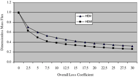
Fig. 3 shows changes in dimensionless mass flux (G/Gmax) with overall loss coefficient for the Test #1. Gmax in the dimensionless mass flux is the calculated mass flux for a perfect nozzle. The mass flux of the HEM is clearly shown to overpredict with larger overall loss coefficients (longer runs of pipe). Predictions from HEM and HEMI indicate there are significant differences. Employing an incompatible mathematical model with fluid physics results in less conservative results as shown in Fig. 3. Thus, it is very important that every homogeneous equilibrium model should be confirmed to satisfactorily represent the flow behavior in pipes both mathematically and physically.
[image:5.595.54.533.480.799.2]
Table V is a summary of prediction results for Sozzi and Sutherland test data on Nozzle 2 with the 1.778 m long straight tube (longest flow length) for low stagnation quality (0.001 < x0 < 0.005) saturated water. The experimental data indicate thermal nonequilibrium because the observed exit pressures are significantly lower than the calculated exit pressures of both of the homogeneous equilibrium models.
Table V
Sozzi and Sutherland Nozzle 2 (L= 1.778 m) Data vs. HEM and HEMI Predictions P0,
MPa
Quality,
x0at P0
Observed
G, kg/m2·s P2, MPa
Calculated HEM
G, kg/m2·s P2, MPa
Calculated HEMI
G, kg/m2·s P2, MPa
Calculated
HEMI Nonequilibrium
G, kg/m2·s P2, MPa
6.867 0.00200 19286 2.455 17884 3.971 15970 3.592 18251 2.413
6.833 0.00280 18358 2.441 17762 3.944 15873 3.565 18128 2.399
6.791 0.00310 17919 2.413 17670 3.916 15790 3.544 18036 2.379
6.757 0.00250 17919 2.379 17660 3.909 15770 3.537 18021 2.379
6.722, Test #1 0.00350 17528 2.379 17518 3.882 15658 3.509 17884 2.358
6.681 0.00330 17528 2.365 17464 3.861 15604 3.496 17826 2.358
6.647 0.00340 17528 2.344 17401 3.840 15546 3.475 17757 2.337
6.605 0.00330 17528 2.344 17338 3.820 15487 3.454 17694 2.324
6.936 0.00188 19334 2.482 18011 4.006 16092 3.627 18382 2.441
6.915 0.00301 19334 2.413 17884 3.985 15990 3.606 18260 2.427
6.902 0.00405 19334 2.351 17777 3.964 15907 3.592 18163 2.413
6.881 0.00428 18309 2.358 17728 3.951 15863 3.578 18109 2.399
6.853 0.00430 17772 2.344 17679 3.937 15819 3.565 18055 2.392
6.826, Test #2 0.00455 17577 2.337 17611 3.923 15760 3.551 17992 2.386
6.860 0.00131 19481 2.448 17928 3.971 16005 3.592 18290 2.420
6.833 0.00162 18944 2.448 17826 3.951 15902 3.565 18177 2.386
6.812 0.00172 18944 2.420 17816 3.944 15902 3.565 18172 2.399
6.784 0.00178 18553 2.427 17762 3.930 15853 3.551 18119 2.386
6.757 0.00177 18553 2.413 17718 3.916 15814 3.537 18075 2.379
6.709 0.00197 18553 2.344 17621 3.889 15726 3.516 17972 2.372
6.709 0.00209 18553 2.330 17611 3.889 15717 3.509 17962 2.358
6.860 0.00240 19334 2.386 17840 3.958 15936 3.585 18207 2.413
6.826, Test #3 0.00240 17870 2.330 17782 3.944 15883 3.565 18148 2.392
6.791 0.00280 17870 2.310 17689 3.923 15809 3.551 18060 2.392
6.757 0.00290 17577 2.310 17640 3.902 15760 3.530 18006 2.372
973 . 0 249 . 1 963 . 0 185 . 3
exp
Although homogenous equilibrium models predict smaller mass flux with lower exit pressure, thermal nonequilibrium ultimately leads to higher flow values. Therefore, it is evident that there is something wrong if the homogeneous equilibrium predictions are quite close to the experimental data. However, preliminary HEMI’s nonequilibrium predictions for both the mass flux and the exit pressure are in good agreement with the experimental data. This also verifies that HEMI is a real homogenous equilibrium model that can be extended to account for the non-equilibrium effects.
VII. CONCLUSION
HEMI has several practical advantages over existing homogeneous equilibrium models: it predicts accurate mass flow capacity and pressure drop for an equilibrium flow using a theoretically developed flow equation which is mathematically and physically satisfactory, it yields conservative results as supposed, and it is simple and easy to apply for all fluids at any conditions. HEMI also offers opportunities to revisit previous experimental data to draw out a better solution for nonequilibrium effects.
REFERENCES
[1] G. L. Sozzi and W. A. Sutherland, “Critical flow of saturated and subcooled water at high pressure,” Report NEDO-13418, General Electric Company, San Jose, CA (July 1975).
[2] “Guidelines for pressure relief and effluent handling systems,” Center for Chemical Process Safety (CCPS), AIChE, New York (1998). [3] R. Darby, P. R. Meiller, and J. R. Stockton, “Select the best model for
two-phase relief sizing,” Chem. Eng. Progress, pp. 56 – 64 (May 2001). [4] L. L. Simpson, “Navigating the two-phase maze” in International
Symposium on Runaway Reactions and Pressure Relief Design, G. A. Melhem and H. G. Fisher, eds., Design Institute for Emergency Relief Systems (DIERS), AIChE, New York, meeting held in Boston, MA, pp. 394 – 417 (August 2-4 1995).
[5] “ASME Boiler and Pressure Vessel Code, Section VIII Div. 1, Pressure Vessels”, American Society of Mechanical Engineers, NY (2007 Edition).
0.0 0.2 0.4 0.6 0.8 1.0 1.2
0 2.5 5 7.5 10 12.5 15 17.5 20 22.5 25 27.5 30 Overall Loss Coefficient
D
im
ens
io
nl
es
s M
as
s
F
lux HEM
[image:6.595.53.291.188.321.2]HEMI