Abstract— Probabilistic methods called Gaussian processes have been successfully shown as a powerful tool for modeling time series data and prediction problem as they are a Bayesian approach with kernel based learning. In this paper, the Gaussian processes are applied to model and predict financial volatility based on GARCH, EGARCH and GJR. Five different kernels are used to train each of the proposed volatility models. More precisely, the experimental results show that, the nonlinear hybrid models can capture well symmetric and asymmetric effects of news on volatility and yields better predictive performance than the classic GARCH, EGARCH and GJR approaches.
Index Terms— Gaussian Process, GARCH, EGARCH, GJR, volatility
I. INTRODUCTION
Financial time series plays a crucial role in modeling and forecasting volatility of stock markets. The most famous and classic models include GARCH, EGARCH, and GJR models, [1,2,3,4] which cover symmetric and asymmetric effects of news in volatility. Since the volatility is very important for portfolio selection, option pricing and risk management, many researchers have used machine learning techniques, for instance, neural network and support vector machine, to improve the prediction of the financial volatility [5]. The main reason of using neural network and support vector machine is their flexible abilities to approximate any nonlinear functions arbitrarily without priori assumptions on data distribution [6]. Hence these approaches can cope with the situation that stock market is most of the time heavy tailed and violates normality. In addition, the neural network can capture the stylized characteristics of financial returns such as leptokurtosis, volatility clustering, and leverage effects; hence it generates better prediction of GARCH family [7]. For comprehensive discussions of GARCH predictions by the support vector machine approach, it is referred to [8,9,10,11].
Manuscript received in July 23, 2010. This work was supported by Shanghai Leading Academic Discipline Project, Project Number: S30504.
P. H. Ou is with School of Business, University of Shanghai for Science and Technology, Rm 101, International Exchange Center, No. 516, Jun Gong Road, Shanghai 200093, China. (Corresponding author, phone: +86- 13661751547; e-mail: [email protected]).
H. S. Wang is with School of Business, University of Shanghai for Science and Technology, No. 516, Jun Gong Road, Shanghai 200093, China. (e-mail: [email protected]).
Gaussian processes (GP) are one of Bayesian non-parametric methods in machine learning whose functional form are the same as the well-known neural network and support vector machine. Like other kernel based methods such as the SVM, they combine a high flexibility of the model by working in high dimensional feature spaces with the simplicity that all operations are kernelized, i.e., they are performed in the lower dimensional input space using positive definite kernel. See [12] for detailed illustration. Besides, the GP have been applied in various areas including human function [13], real time online model [14], classification [15], non-stationary time series prediction [16], and dynamic model for human motion [17].
Inspired by such efficiently predictive capability of the Gaussian processes and their successful applications, we are very interested in applying it for volatility prediction. Therefore, it is valuable for us to research the problem of whether more accurate forecasting performance could be achieved if we combine the GP with GARCH, EGARCH, and GJR structures to construct new hybrid models of financial volatility, say GARCH, EGARCH and GP-GJR.
In this work, simulated and real data, NASDAQ index, are analyzed to validate the proposed models. Five different kernels (or covariance functions) are applied to each of the volatility models as they are the heart of obtaining the Gaussian processes. The paper is organized as follow. Next section introduces volatility models based on classical GARCH, EGARCH, GJR and hybrid Gaussian Processes with GARCH, EGARCH and GJR. Section 3 presents the experimental results including parameters estimation, Gaussian Processes training and out of sample forecasting performance. The last section is reserved for conclusion.
II. VOLATILITY MODELING
A. Parametric models
Let be stock price at time . Then
100 (1)
denotes the continuously compounded daily returns of the underlying assets at time .
GARCH(1,1) is defined as , , and (2) where 0 , 0 , 0, and this process is weakly stationary if 1. is a sequence of (iid) independent identically distributed random variables with mean 0 and variance 1. One step ahead forecast of
GARCH(1,1) is .
Modeling and Forecasting Stock Market
Volatility by Gaussian Processes based on
GARCH, EGARCH and GJR Models
GJR(1,1) is written as the following:
(3) where 1 for 0 and 0 otherwise. Stationary assumption for the model requires 1, 0, 0 , 0, 0. The model assumes that bad news have higher impact than the good news. One
step-ahead-forecast for GJR(1,1) is for
0 and for 0.
EGARCH(1,1) is represented as logarithm form:
| | | |
(4) EGARCH model allows good news and bad news to have a different impact on volatility because the level of is included with a coefficient . One step ahead forecast by EGARCH(1,1) is
| |
.
B. Hybrid models of GARCH, EGARCH and GP-GJR
Gaussian Processes based on GARCH, EGARCH and GJR models are represented as
GP-GARCH: , ∗ (5) where is treated as dependent variable, and ,
∗ are treated as independent variables. Its one step ahead forecast is , ∗ .
GP-GJR model: , ∗ , ∗∗ (6) where the input variables are defined as ,
∗ and ∗∗ . One step ahead forecast of this model is , ∗, ∗∗ .
GP-EGARCH: , ∗ , ∗∗ (7) where is treated as response. The regressors, in this
case, are denoted as , ∗ | |
| |
and ∗∗ . Here the expected value | |
is approximated by its mean value. One step ahead forecast based on GP-EGARCH is defined as exponential transformation: , ∗, ∗∗ .
Note, for all models, we take assuming 0 (as usual) and ∑ according to [8] so that we can obtain , ∗ , ∗∗ and before making analysis. The function is approximated by the Gaussian Processes in (10) below to be .
C. Gaussian Processes
Gaussian processes are a popular method for nonparametric regression. Gaussian processes are defined by its mean and covariance functions. It is assumed that the observations are normally distributed. Using the kernel matrix as the covariance matrix is a convenient way of extending Bayesian modeling of linear estimators to nonlinear situations. Furthermore, it represents the counterpart of the kernel trick in methods minimizing the regularized risk. Specifically, given a set of training data , , 1, … , , the objective is to predict the value of new ∗given ∗ via a learning function such
that where is normally distributed with mean zero and variance . With the assumption of the Gaussian noise, , the observed target can be described as ~ 0, , where , denotes the covariance matrix and is matrix of input. The common choice of covariance function is a Gaussian kernel defined as
, (8)
where denotes the signal variance and Ware the widths of the Gaussian kernel.
For a new ∗, the predictive distribution of the corresponding outputs is simply obtained by conditioning on the training data to obtain ∗ | ∗ , . The joint distribution of the observed target values and predicted value for ∗ is given by
∗ ~ 0 ,
, , ∗
∗, ∗, ∗ . (9) The conditional distribution is also Gaussian and yields the predicted mean value ̅ ∗ with the variance ∗ ,
̅ ∗ ∗ ∗ (10)
∗ ∗, ∗ ∗ ∗ (11)
where k*k(X,x*),KK(X,X)and denotes the so-called prediction vector.
The predicted mean ̅ ∗ is in general used as an estimate of the output ∗ with uncertainty ∗ . The hyper-parameters of Gaussian processes with their kernel and their optimal value for a particular data set can be derived by maximizing the log marginal likelihood using common optimization procedures such as Quasi-Newton methods.
Five different kernels (or covariance functions) used in this study includes
- Gaussian radial basis function
, ‖ ‖ (12)
- Linear kernel which is simplest case:
, 〈 , 〉 (13) - Polynomial kernel:
, scale ∙ 〈 , 〉 offset (14) - Laplace radial basis kernel:
, ‖ ‖ (15) - Bessel function:
,
‖ ‖ . (16)
III. EMPIRICAL ANALYSIS
A. Artificial Simulated Data
In this section, we investigate the forecasting performance of all models using simulated data. We generate 1000 samples from GARCH(1,1) with coefficients 0.0001,
0.01, 0.1, 0.8 and EGARCH(1,1) 0.0001, 0.01, 0.1, 0.8, 0.06 as well
0.06 with, first, Normal innovation and then the Student’s t with 6 degree of freedom. The second innovation distribution tries to model the excess of kurtosis that usually appears in real financial time series. Six sets of simulated data are achieved and then fitted by hybrid models based on the GP as in (5), (6), and (7). These simulated data are also fitted again, respectively, by six different models of GARCH, EGARCH and GJR with Normal and Student’s innovations to make comparison with the hybrid approaches. 75% of the whole data, 750 observations, are used for estimation or training the models; and the remaining data, 250 points, are reserved for out of sample forecasting. GARCH toolbox in Matlab is used to simulate the return series and to fit GARCH, EGARCH and GJR models; and Kernlab package in R software by [18] is used to fit the volatility models based on the Gaussian processes.
TABLE I
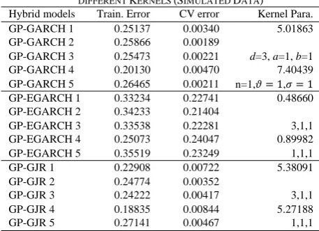
TRAINING RESULTS BY GAUSSIAN PROCESS WITH FIVE DIFFERENT KERNELS (SIMULATED DATA)
Hybrid models Train. Error CV error Kernel Para.
GP-GARCH 1 0.25137 0.00340 5.01863
GP-GARCH 2 0.25866 0.00189
GP-GARCH 3 0.25473 0.00221 d=3, a=1, b=1
GP-GARCH 4 0.20130 0.00470 7.40439
GP-GARCH 5 0.26465 0.00211 n=1, 1, 1
GP-EGARCH 1 0.33234 0.22741 0.48660 GP-EGARCH 2 0.34233 0.21404
GP-EGARCH 3 0.33538 0.22281 3,1,1
GP-EGARCH 4 0.25073 0.24047 0.89982
GP-EGARCH 5 0.35519 0.23249 1,1,1
GP-GJR 1 0.22908 0.00722 5.38091
GP-GJR 2 0.24774 0.00352
GP-GJR 3 0.24222 0.00417 3,1,1
GP-GJR 4 0.18835 0.00844 5.27188
GP-GJR 5 0.27141 0.00467 1,1,1
Note: 1. GP-GARCH 1, 2, 3, 4, 5 denote Gaussian Process based on GARCH with Gaussian Kernel, Linear kernel, Polynomial kernel, Laplace Kernel, and Bessel kernel respectively. 2. CV error = 10 fold Cross Validation error.
3. a is scale, b is offset and d is degree of the polynomial kernel.
TABLE II
OUT OF SAMPLE FORECASTING PERFORMANCE (SIMULATED DATA) Simulated
GARCH(1,1)
Normal innovation Student’s Innovation
NMSE NMSE
GARCH-N,T 0.97330 0.1505 0.97040 0.1499 GP-GARCH1 0.74431 0.2626 0.98552 0.0260
GP-GARCH2 0.70946 0.3022 0.69233 0.3341
GP-GARCH3 0.69732 0.3161 0.70326 0.3216
GP-GARCH4 0.80456 0.1974 0.99819 0.0188 GP-GARCH5 0.69627 0.3226 0.80097 0.2038 Simulated
EGARC(1,1)
Normal innovation Student’s Innovation
NMSE NMSE
EGARC-N,T 0.94444 0.0900 0.92210 0.1093
GP-EGARC1 0.70897 0.3300 0.87006 0.1618
GP-EGARC2 0.74054 0.2820 0.79103 0.2599
GP-EGARC3 0.71590 0.3224 0.54061 0.5315
GP-EGARC4 0.71949 0.3177 0.87476 0.1534 GP-EGARC5 0.72364 0.2998 0.85129 0.1936 Simulated
GJR(1,1)
Normal innovation Student’s Innovation
NMSE NMSE
GJR‐N,T 0.89345 0.1068 0.76465 0.1562
GP-GJR 1 0.83414 0.1630 0.97703 0.0290 GP-GJR 2 0.64595 0.3738 0.66360 0.3601
GP-GJR 3 0.63715 0.3833 0.58039 0.4437
GP-GJR 4 0.87530 0.1280 0.97189 0.0415 GP-GJR 5 0.67596 0.3332 0.94129 0.0603 Note: is obtained by regression between actual volatilities (square returns) and predicted volatilities. NMSE stands for normalized mean squared error.
In this experiment, 70% of the training data is used for training the GP model to get the optimal hyper-parameter of Kernel (or correlation) function and the remaining data, 30%, is reserved for validation of the model. The optimal results of the training, including the training error, 10 fold cross-validation error and Kernel parameter, are displayed in Table I. The training results of GP from simulated data for GARCH, EGARCH and GJR based returns with Student’s t innovation are not shown here to reduce the space. The forecasting performance from each model for out-of-sample data, measured by NMSE and , are shown in Table II. Basically, the larger value, the better the model predicts the actual values. The smaller value of NMSE, the more preferred the model. From the Table II, it is seen that most of the hybrid models yield more accuracy than the parametric models.
B. Real data of NASDAQ index
Now we analyze NASDAQ index, , which is first downloaded from the Yahoo finance and then transformed into log return as in (1). The whole sample consists of 3274 daily data spanning from 02 Jan. 1996 to 31 Dec. 2008 which covers the financial crisis period. We select subsample of size 3023, dated from 02 Jan. 1996 to 31 Dec. 2007, as the training set for the Gaussian Processes or parameter estimation for classic models. The remaining sample of size 251 daily data, Jan-Dec 2008, is used as the test set or for out-of-sample forecasting. Table III summarizes the descriptive statistics of the index return series along the whole period.
TABLE III
SUMMARY STATISTIC (NASDAQ)
Sample 3274 Excess Kurtosis 4.57513
Mean 0.0132 LB.Q2 3057.27
Std.Dev. 1.7998 JB test 2861.30
Skewness -0.01079 ARCH(12) 648.367
We remark that these facts suggest a highly competitive and volatile market. There are significant price fluctuations in the markets as suggested by positive standard deviation. The negative skewness indicates that there is a high probability of losses in the market. The excess value of kurtosis suggests that the market is volatile with high probability of extreme events occurrences. Moreover, the rejection of Jarque Bera (JB) test of normality shows that the returns deviate from normal distribution significantly and exhibit leptokurtic. The Ljung Box statistic for squared return and Engle ARCH test prove the exhibition of ARCH effects in the return series. Therefore, it is appropriate to apply GARCH, EGARCH, GJR especially the hybrid approach for modeling volatility to this return.
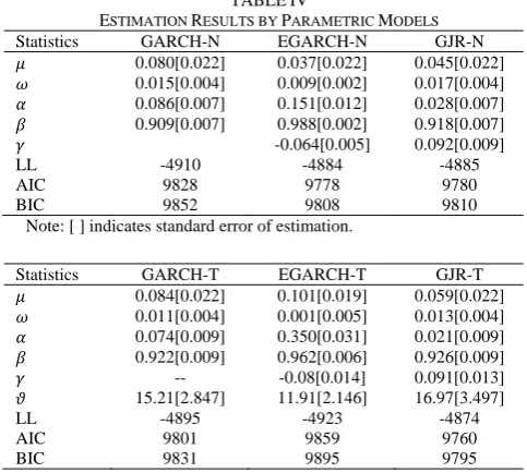
We, then, apply the return series to (2), (3) and (4) to get parameters of GARCH, GJR and EGARCH models with normal and student’s t innovations. The estimation results and diagnosis are shown in Table IV. Among the parametric models, the series best fit to the GJR with student’s t innovation, GJR-T, according to highest value of Log likelihood (LL) and smallest value of AIC and BIC. The conditions of asymmetric effects hold for all models according to the significance of leverage effect coefficients
[image:3.595.46.275.269.435.2] [image:3.595.45.278.523.760.2]TABLE IV
ESTIMATION RESULTS BY PARAMETRIC MODELS
Statistics GARCH-N EGARCH-N GJR-N 0.080[0.022] 0.037[0.022] 0.045[0.022] 0.015[0.004] 0.009[0.002] 0.017[0.004] 0.086[0.007] 0.151[0.012] 0.028[0.007] 0.909[0.007] 0.988[0.002] 0.918[0.007]
-0.064[0.005] 0.092[0.009]
LL -4910 -4884 -4885
AIC 9828 9778 9780
BIC 9852 9808 9810
Note: [ ] indicates standard error of estimation.
Statistics GARCH-T EGARCH-T GJR-T 0.084[0.022] 0.101[0.019] 0.059[0.022] 0.011[0.004] 0.001[0.005] 0.013[0.004] 0.074[0.009] 0.350[0.031] 0.021[0.009] 0.922[0.009] 0.962[0.006] 0.926[0.009]
-- -0.08[0.014] 0.091[0.013]
15.21[2.847] 11.91[2.146] 16.97[3.497]
LL -4895 -4923 -4874
AIC 9801 9859 9760
BIC 9831 9895 9795
Note: [ ] indicates standard error of estimation.
TABLE V
TRAINING RESULTS BY GAUSSIAN PROCESSES
Hybrid models Train. Error CV error Kernel Para.
GP-GARCH 1 0.20629 16.1661 42.56467
GP-GARCH 2 0.15063 4.00422
GP-GARCH 3 0.14506 3.71741 3, 1,1
GP-GARCH 4 0.21857 19.8882 49.10658
GP-GARCH 5 0.18365 6.81695 1, 1, 1
GP-EGARCH 1 0.13332 0.19156 0.64779
GP-EGARCH 2 0.13863 0.18574
GP-EGARCH 3 0.13386 0.18165 3, 1, 1
GP-EGARCH 4 0.11323 0.18973 0.59678
GP-EGARCH 5 0.13836 0.18820 1, 1, 1
GP-GJR 1 0.21351 17.3607 33.09276
GP-GJR 2 0.14812 3.53482
GP-GJR 3 0.13935 16.4461 3, 1, 1
GP-GJR 4 0.21810 19.8230 30.89865
GP-GJR 5 0.18494 7.74181 1, 1, 1
Note: 1. GP-GARCH 1, 2, 3, 4, 5 denote Gaussian Process based on GARCH with Gaussian Kernel, Linear kernel, Polynomial kernel, Laplace Kernel, and Bessel kernel respectively.
2. CV error = 10 fold Cross Validation error.
[image:4.595.45.287.55.272.2]Now we train Gaussian processes to the return series by (5) for GARCH, (6) GJR and (7) for EGARCH. The optimal results of the training, including the training error, 10 fold cross-validation error and Kernel parameter, are displayed in Table V. These volatility models are used to forecast future volatilities in the test set for comparison with the classic models. Table VI report the values of NMSE and obtained from different models. The Gaussian processes achieve smallest value of NMSE and highest value of . This implies that the Gaussian Processes method can capture well both symmetric and asymmetric volatilities and also produce improved forecasting performance than the parametric models. Fig. 1,2,3 also plot the superior performance of the Gaussian Processes in modeling and forecasting volatilities based on GARCH (Fig.1) and EGARCH forms (Fig.2) as well as GJR types (Fig.3). It is seen that the forecasting lines by the hybrid models, GP-GARCH, GP-EGARCH and GP-GJR, are more flexible and can capture more extreme points than the corresponding classic models.
TABLE VI
OUT OF SAMPLE FORECASTING PERFORMANCE (NASDAQ) NMSE
GARCH-N 0.7925 0.2163
GARCH-T 0.8105 0.1949
GP-GARCH1 0.6995 0.3353
GP-GARCH2 0.5576 0.4513
GP-GARCH3 0.5599 0.4483
GP-GARCH4 0.6965 0.3719
GP-GARCH5 0.6277 0.3847
EGARCH-N 0.8013 0.1961
EGARCH-T 0.6233 0.3934
GP-EGARCH1 0.6741 0.3387
GP-EGARCH2 0.5958 0.4259
GP-EGARCH3 0.5769 0.4392
GP-EGARCH4 0.6521 0.3626
GP-EGARCH5 0.6904 0.3442
GJR-N 0.7782 0.2317 GJR-T 0.7886 0.2188
GP-GJR1 0.7081 0.2899
GP-GJR2 0.5586 0.4500
GP-GJR3 0.5621 0.2965
GP-GJR4 0.6971 0.3701
GP-GJR5 0.6471 0.3693
Note: is obtained by regression between actual volatilities (square returns) and predicted volatilities. NMSE stands for normalized mean squared error.
IV. CONCLUSION
In this paper, we proposed nonlinear volatility models based on Gaussian processes combined with GARCH, EGARCH and GJR models. The empirical analysis of simulated and real data, NASDAQ index, show that these hybrid models can capture well the symmetric and asymmetric effects of news in volatility and generate superior performance of volatility prediction than the corresponding classic models of GARCH, EGARCH and GJR with both Normal and Student’s t innovations. Among the five kernels, Linear and Polynomial kernels are most suited for the hybrid Gaussian processes in this study. In addition, the Gaussian process models are simple, practical and powerful Bayesian tools for data analysis.
ACKNOWLEDGMENT
We appreciate referees for comments on our work. REFERENCES
[1] R. F. Engle, “Autoregressive conditional heteroskedasticity with estimates of variance of UK inflation”, Econometrica, vol. 50, no. 4, pp. 987-1008, 1982.
[2] T. Bollerslev, “Generalized Auto Regressive Conditional Heteroskedasticity”, Journal of Econometrics, vol. 31, no. 3, pp 307-327, 1986.
[3] D. B. Nelson, “Conditional Heteroskedasticity in Asset Returns: A New Approach”, Econometrica, vol. 59, no. 2, pp. 347-370, 1991. [4] L. Glosten, R. Jagannathan, and D. Runkle, “On the relationship
between the expected value and the volatility of the nominal excess return on stocks”, Journal of Finance, vol. 48, no. 5, pp. 1779-1801, 1993.
[5] R. G. Donaldson, and M. Kamstra, “An artificial neural network-GARCH model for international stock return volatility”, Journal of Empirical Finance, vol. 4, no. 1, pp. 17-46, Jan. 1997.
[6] S. Haykin, Neural networks: a comprehensive foundation, Englewood cliffs: Prentice Hall, 1999.
[image:4.595.44.285.311.472.2]returns in Istanbul Stock Exchange”, Expert Systems with Applications, vol. 36, no. 4, pp. 7355-7362, May 2009.
[8] F. Perez-Cruz, J. A. Afonso-Rodriguez, and J. Giner, “Estimating GARCH models using support vector machines. Quantitative Finance, vol. 3, no. 3, pp 163-172, Jun. 2003.
[9] L. B. Tang, H.Y. Sheng, and L.X. Tang, “Forecasting volatility based on wavelet support vector machine”, Expert Systems with Applications, vol. 36, no. 2, pp. 2901-2909, Mar. 2009.
[10] L. B. Tang, H. Y. Sheng, and L. X. Tang, “GARCH prediction using spline wavelet support vector machine”, Neural Computing and Application, vol. 18, no. 8, pp. 913-917, Feb. 2009.
[11] S. Chen, K. Jeong, & W. Hardle, “Forecasting volatility with support vector machine-based GARCH model”, Journal of Forecasting, vol. 29, no. 4, pp. 406-433, Sep. 2009.
[12] C. E. Rasmussen and C. K. I. Williams, Gaussian Processes for Machine Learning, Massachusetts: the MIT Press, 2006.
[13] T. L. Griffiths, C. Lucas, J. Williams, and M. L. Kalish, “Modeling human function learning with Gaussian processes”, in Proc. 22nd Annu. Conf. on Neural Information Processing Systems Foundation, Berkeley, 2008.
[14] D. Nguyen-Tuong, M. Seeger and J. Peters, Real-Time Local GP Model Learning, O. Sigaud, J. Peters(Eds): From Motor Learning to Interaction Learning in Robots, Studies in Computational Intelligence, vol. 264, pp. 193-207, 2010.
[15] C. K. I. Williams & D.Barber, “ Bayesian Classification with Gaussian Processes”, IEEE Trans. Pattern Analysis and Machine Intelligence, vol. 20, no. 12, pp. 1342-1351, 1999.
[16] S. Brahim-Belhouari, and A. Bermak, “Gaussian process for nonstationary time series prediction”, Computational Statistics & Data Analysis, vol. 47, no. 4, pp. 705-712, Nov. 2004.
[17] J. M. Wang, D. J. Fleet and A. Hertzmann. “Gaussian Process Dynamical Models for Human Motion”, IEEE Transactions on Pattern Analysis and Machine Intelligence, vol. 30, no. 2, pp. 283-298, Feb. 2008.
[18] A. Karatzoglou, A. Smola., A. Hornik and A. Zeileis. (2004). An S4 Package for Kernel Methods in R. Journal of Statistical Software, [Online].11(9). Available: http://www.jstatsoft.org/
APPENDIX
The NMSE is defined as NMSE ∑ where
∑ . Here we take as actual
values, and is treated as the forecasted volatility obtained by each of the competing models. is sample size corresponding to each time of forecasting. The square correlation is a measure of forecasting performance is obtained by regressing squared return on a constant and the forecasted volatility for out-of-sample time point, 1,2, … , , . In this regression, the constant term should be close to zero and the slope should close to 1. The higher value of , the better the forecasting model.
FIGURE 1. . PLOT OF VOLATILITY BASED GARCH VERSUS GP-GARCH
FIGURE 2. . PLOT OF VOLATILITY BASED EGARCH VERSUS GP-EGARCH
FIGURE 3. PLOT OF VOLATILITY BASED GJR VERSUS GP-GJR
0 50 100 150 200 250
0 2 4 6 8 10 12
Volatility forecasts by GARCH VS GP-GARCH models
Actual GARCH GP-GARCH
0 50 100 150 200 250
0 2 4 6 8 10 12
Volatility forecasts by EGARCH VS GP-EGARCH
Actual EGARCH GP-EGARCH
0 50 100 150 200 250
0 2 4 6 8 10 12
Volatility forecasts by GJR VS GP-GJR models