Abstract— Modeling road accidents using panel data
approach recently has gained wide attention and application. As the nature of road crashes are non-negative count, the traditional linear computational approaches is inappropriate giving the nonlinear model of fixed effects (FE) the better choice. This paper examines the road accidents relationship with precipitation factors by estimating the FE Negative Binomial (NB) model. In the FE model two estimation methods were consider in this paper: conditional and unconditional estimation method. Thus, this paper compare the conditional and unconditional FE model for road accidents and discuss the findings obtain. Results showed that the unconditional FE Negative Binomial model gives approximately the same results with conditional models. The effect of monthly rainfall with shorter spell period presents greater risk of accident rate. On the other hand, a negative relationship is found between the monthly rainfalls with longer spell period and accident rate.
Index Terms— Conditional Fixed Effects, Unconditional
Fixed Effects, Negative Binomial, Road accidents
I. INTRODUCTION
VER the past few years road accidents represent among the leading cause of death and injury. Statistics recorded had captured the interest of the researcher and policy maker to better understand the complexity of factors that are related to road accidents by developing statistical model. Models developed served as references for law enforcement agencies and policy maker to implement corrective action aimed to reduce the number of road accidents. Thus, there has been considerable research conducted on the development of statistical model for predicting road accident crash. A detailed review on advancement of methodological approach in crash frequency data can be found in Lord and Mannering [1]. Despite numerous advancement in estimation tools of statistical model for count data, the most common probabilities structure used for modeling road accident
Manuscript received March 6, 2012; revised April 12, 2012. This work was supported in part by the Ministry of Higher Education, Malaysia under Grant FRGS/2/2010/SG/UITM/02/34.
W. F. W. Yaacob is with Faculty of Computer and Mathematical Sciences, UiTM Shah Alam, 40450 Shah Alam, Selangor, Malaysia. (corresponding author: phone: +6019-985-3350; fax: +603-5543-5503; e-mail: [email protected]).
M. A. Lazim is with Faculty of Computer and Mathematical Sciences, UiTM Shah Alam, 40450 Shah Alam, Selangor, Malaysia. (email: [email protected])
Y. B. Wah is with Faculty of Computer and Mathematical Sciences, UiTM Shah Alam, 40450 Shah Alam, Selangor, Malaysia. (email: [email protected])
remains the traditional Poisson and Negative Binomial distribution. When dealing with panel data type of road accident count, the most familiar panel data treatments are the fixed effects (FE) and the random effects (RE) which were proposed for panel count data model by Hausman, Hall and Griliches (HHG) [2]. We employed the panel model approach of fixed effects negative binomial model method since it has several advantages over individual time series and cross sectional model [3],[4], particularly, for its ability to account for heterogeneity in the data [5]. Since, many studies had proven that precipitation generally results in more accidents compared with dry condition [6]-[8], therefore, in this study we will examines the relationship between road accidents and various precipitation factors.
Given the discrete, non-negative nature of the road accidents count, the ordinary least square is not appropriate to model this type of data [9]. Hence, the HHG negative binomial model based on conditional estimation method was employed first. Though analysis on the HHG Poisson FE is simple and has been recognized to be exceptional from incidental parameter problem [10],[11], the HHG formulation of conditional NB FE model is ambiguous [12], [13]. Thus, to account for this ambiguity in HHG FE NB, we also consider the unconditional FENB model [14]. The various models developed were applied in road accident panel data set which allows for a detailed discussion and comparison.
In section 2 we review some related works on the application of the model. Section 3 presents the models and its properties. Application to examine the relationship of road accident and precipitation factors using conditional and unconditional FE NB is presented in Section 4. Results and discussions are presented in Section 5. Finally, the last section discussed the policy lessons.
II. RELATED WORK
The literature on panel count model has grown considerably after the seminal work of Hausman, Hall and Grilliches (HHG) et al. [2]. Application of panel count model can be seen in varieties of application [15], [16]. Panel models have also become popular in road safety literature. Previous work on panel count model in road accident application has been widely applying both fixed effects and random effects model as suggested by Hausman et al. [4], [5],[ 7].
Eisenberg [7] examined the relationship between precipitation and traffic crashes in 48 contiguous states in US using fixed effects negative binomial model for the period of 1975 to 2000. It was found that precipitation is
Modeling Road Accidents using Fixed Effects
Model: Conditional versus Unconditional Model
Wan Fairos Wan Yaacob, Mohamad Alias Lazim and Yap Bee Wah
positively associated with fatal crashes. In terms of dry spell effects, this study found that the rainfall amount has enhanced effects on accident count after a dry spell due to the slippery surface from accumulation of oil on the roads.
Based on 6-year crash data set for urban and suburban arterial of 92 counties in Indiana, Karlaftis and Tarko [4] employed fixed effects model of Poisson and negative binomial to develop the crash model. Their findings indicated that the increase in the number of accidents is associated with higher vehicle miles travelled, population, the proportion of city mileage, and the proportion of urban roads in total vehicle miles travelled.
Kweon and Kockelman [17] investigated the safety effects of the speed limit increase on crash count measure in Washington State using the panel regression methods of both the fixed effects and random effects model assumption. They develop models for the number of fatalities, injuries, crashes, fatal crashes, injury crashes, and property-damage-only (PDO) crashes using fixed effects and random effects Poisson and negative binomial model specification. They found that the fixed-effects negative binomial model performed best in describing injury count while for fatalities, injuries, PDO crashes and total crashes, the pooled negative binomial model was a better choice.
There is also another study that applied fixed effects negative binomial model in the analysis. Kumara and Chin [18] analyzed the fatal road accident data from the period of 1980 to 1994 across 41 countries in the Asia Pacific region and found that road network per capita, gross national product, population and number of registered vehicles were positively associated with fatal accident occurrence.
In another recent study, Law et al. [5] examined the effect of motorcycle helmet law, medical care, technology improvement, and the quality of political institution on motorcycle death on the basis of Kuznets relationships. They used the HHG fixed effects negative binomial model on a panel of 25 countries from the period of 1970 to 1999. Their findings revealed that implementation of road safety regulation, improvement in the quality of political institution and medical care and technology developments showed significant effect in reducing motorcycle death.
III. METHODOLOGY
This section discusses the formulation of panel count model specification of the fixed effects Negative Binomial model for both conditional and unconditional approach.
A. Conditional estimation of Fixed Effects Negative Binomial Model
The estimation method used in this study is the panel negative binomial regression developed by Hausman et al. [2], a generalized version of Poisson regression that allows the variance of dependent variable to differ from its mean. The model can be expressed in the following way;
( )
(
)
ln lit =ai+ln Vehit +gTimeit+b¢Xit+eit (1) for i=1, 2,...N and t=1, 2 ,...Ti
where
l
it is the dependent variable of road accident count for a given observation subscripted by state and time; ai is the state specific effects;b g
, are the model parameter;Time is the time trend; Xitincludes other independent
variables of interest;
e
is the error term. To illustrate the fixed effect negative binomial model, Hausman et. al [2] add individual specific effects of aiand the negative binomial overdispersion parameter of fiinto the model replacing q a fi = i i . Here, the number of accident, yit fora given time period,
t
is assumed to follow a negative binomial distribution with parameters a li it and fi, wherelit =exp x( )
it¢b giving yit has a mean a l fi it i andvariance
(
a l fi it i) (
´ +1 a fi i)
[9]. This model allows thevariance to be greater than mean. The parameter ai is the individual-specific fixed effects and the parameter fiis the negative binomial overdispersion parameter which can take on any value and varies across individuals. Obviously
i
a and i
f can only be identified as the ratio of a fi i and this ratio has been dropped out for conditional maximum likelihood [10].
The conditional approach of fixed effects Negative Binomial model estimates the parameter b using the conditional joint distribution conditioning on the groups total counts by maximizing the conditional joint distribution as below;
(
)
( ) (
)
i
i
T T
it it
T
t 1 t 1
i1 iT it T T
t 1 i
it it t 1 t 1 T
it it t 1 it it
y 1
P y ,..., y y
y y
y 1
l
l
l l
= =
=
= =
=
æ ö æ ö
Gç ÷ çG + ÷
æ ö è ø è ø
=
ç ÷ æ ö
è ø G +
ç ÷
è ø
G +
´
G G +
å
å
å
å
å
Õ
(2)
The fixed effects model for Poisson distribution does not allow for an overall constant [10]. However, an overall constant term is identified in the conditional distribution of HHG NB formulation [17] indicating that HHG formulation of FE NB model does not formulate the true fixed effects model in the mean of random variable and conditioned out of the distribution to produce the estimated model [13], [19]. Hence, this study also considers the unconditional estimator for both NB FE model.
B. Unconditional estimation of Fixed Effects Negative Binomial Model
(
)
(
)
(
)
1 1
exp exp exp log
!
it i
y T
N i it i it
i t it
Log L
y
a b a b
= =
é ¢ é ¢ ù ù
- + +
ê êë úû ú
= ê ú
ê ú
ê ú
ë û
å Õ
x x(3)
with respect to all K N+ parameters [14], [19]. While the unconditional FE NB model was estimated using the same approach by replacing the Poisson density with the NB counterpart of
(
1,...,)
( )
(
(
)
)
.(
1)
1it
y it
i iT it it it
it y
P y y u u
y q q
q
G +
=
-G G +
x
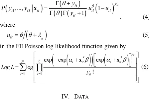
. (4) where
(
it)
it
u =q q l+ (5) in the FE Poisson log likelihood function given by
(
)
(
)
(
)
1 1
exp exp exp log
!
it i
y T
N i it i it
i t it
Log L
y
a b a b
= =
é ¢ é ¢ ù ù
- + +
ê êë úû ú
= ê ú
ê ú
ê ú
ë û
å Õ
x x (6)IV. DATA
In this paper we worked on road accident panel data comprising of a balanced panel monthly data in Peninsular Malaysia from January 1997 to December 2007. The number of observation per states was 132 with a total number of 1584 observations from 12 states. The list of states included in the study is presented in Table 1.
The monthly total road accidents or road crash data were collected from the Royal Malaysian Police Headquarters in Kuala Lumpur for the year 1997 to 2007 [20]. The data used referred to the total figure of their occurrences on public or private roads due to the negligence or omission by any party concerned (on the aspect of road users conduct, maintenance of vehicle and road condition), environmental factor (excluding natural disaster) resulting in a collision (including “out or control” cases and collision of victims in a vehicle against object inside or outside the vehicle e.g. bus passenger) which involved at least one moving vehicle whereby damage or injury was caused to any person, property, vehicle, structure, or animal.
Data on the number of registered vehicles (VEH) were also used which were collected from the Department of Road Transport in the Malaysian Ministry of Transportation. The number referred to the total number of vehicles (private and public) that was registered with the Department of Road Transport. It included all vehicles using either petrol or diesel which were motorcycles, motorcars, buses, taxis and hired cars, goods vehicle and other vehicles. However, the figure did not include army vehicle.
Data for precipitation variables were collected from the Malaysian Meteorological Department (MMD). The precipitation factor considered was the amount of monthly rainfall (in millimeter) for a particular month. The data were captured from 12 selected weather stations in the respective 12 states. This factor had been most commonly
used in previous work in road safety modeling literature [6]-[8].
Another climate factor considered was the number of rainy days (in days) for a particular month. The number of rainy days per month had been considered in previous studies of its relationship with road accident crash [7], [8]. Variation in the number of rainy days could be associated with frequent expose of rain to road user [21]. Hence the number of rainy days was also used in this study. The data were also collected from the Malaysian Meteorological Department (MMD) submitted by the same 12 selected weather stations for rainfall amount data.
Another precipitation factor was the spell effects. The dry spell effect took place when a consecutive series of days without rainfall was broken by the first rain after that period [8]. This study used the spell period that referred to the period of first rain occured since the last rain in a month that may take few days or few weeks as determined by the rainfall recorded at 12 selected weather stations as in Table 1. The spell durations of gap between rain and no-rain were broken down into the following category: (i) 1-7 days; (ii) 8-14 days; (iii) 15-21 days; (iv) 22-28 days and (v) more than 28 days category. Then, the frequency of dry spell for each spell period was obtained for the particular month. If the highest frequency with the highest total number of no-rain day for the particular month fell within the specified spell interval, then the dummy assigned was equal to 1 and the other spell interval dummy would be 0. Note that the dummy for each spell period was mutually exclusive. This dummy was then interacted with the precipitation (rainfall) variable and the interaction term was included as an independent variable. These variables were created to examine what was the effect of this month precipitation with different spell period on this month crash. Thus, the accident counts were regressed with a list of interaction variables between precipitation (rainfall) and dry spell dummy.
TABLEI
THE LIST OF STATES, WEATHER STATION AND YEAR OF DATA
No
. State Station Period
1 Perlis (PL) Chuping 1997 – 2007
2 Kedah (KD) Alor Setara 1997 – 2007 3 Pulau
Pinang
(PP) Bayan Lepas 1997 – 2007
4 Perak (PR) Ipoh 1997 – 2007
5 Selangor (SL) Petaling Jaya 1997 – 2007 6 Kuala
Lumpur
(KL) Parlimenb 1997 – 2007
7 Negeri Sembilan
(NS) Hospital
Serembanc 1997 – 2007
8 Melaka (ML) Melaka 1997 – 2007
9 Johor (JH) Senai 1997 – 2007
10 Pahang (PH) Kuantan 1997 – 2007
11 Terengganu (TR) Kuala Terengganu Airport
1997 – 2007
12 Kelantan (KN) Kota Bharu 1997 – 2007 Weather data (state-day and therefore state-month) are missing for period:
a19-26 Dec 2005; b1-3 Aug 2004; c 1 Jun-15 Oct 2000, 16 May 2001-5Jun
[image:3.595.47.288.174.335.2]Missing observations for rainfall amount and dry spell were calculated by linear interpolation as suggested by previous study [5]. Extrapolations were only done for short period of missing value by averaging the observations over preceding and posterior year.
In addition, the independent variables also included a vector of dummy variables for all state (less one) representing fixed effects for each state and month dummy. The log of the total number of registered vehicle was incorporated in the model as an offset variable. The “offset” term referred to the amount of exposure for a given observation [7]. The risk of accident is not equal for each state. For instance, state with larger vehicle population size will experience more accident than the state with less vehicle size. The different level of risk exposure can be normalized by creating a rate [22]. The rate can be included in the model by introducing the logged form of measure of risk exposure as an offset variable. Hence, the logarithm number of registered vehicle was chosen as the offset variable in this study. The coefficient of independent variables will be interpreted as effects on rates rather than count.
V. RESULTS AND DISCUSSIONS
Table 2 presents the summary statistics for all variables included in the study. Table 3 presents the pairwise correlation coefficients for the main variables used in this analysis. The highest correlation was 0.9509 for rainfall amount and interaction effect for 1 – 7 days dry spell period
and rainfall. The model in Table 4 was estimated without rainfall variable to cater for multicollinearity. The second highest of correlation was 0.654 for rainfall amount and number of rainy days. Table 4 presents the results for negative binomial FE model specification. Both conditional and unconditional model were then estimated and compared. The specification was explored by including all explanatory variables in a linear form of the exponential function. The interpretation of the effect from exponential transformation used in panel count model (to ensure non-negativity) is not as simple as in linear model. In exponential case, E yéë it xitù =û exp
( )
xit¢b and eachvariable’s marginal effects are as follows;
( )
exp
it it
it j it it j
ji
E y
E y
b b b
é ù
¶ ë û= ¢ ´ = é ù´
ë û
¶ x
x x
x [12] which
implies that a unit change in the jth variable leads to a multiplicative change in E yéë it xitùû of bj. The coefficients
represent the effect of independent variables on the log of the mean of dependent variable which can be interpreted as percentage changes in the expected count or rate for 1 unit increase in the independent variable.
The increase in the number of rainy days is predicted to result in higher accident rate. The adverse effects are estimated to be 1, which is the number of increase of rainy days in a month associated with 0.3 percent increase in the monthly accident rate. This result is in accordance with the
TABLEIII
CORRELATION MATRIX
ARain RainyD Time Spell_1-7 Spell_8-14 Spell_15-21 Spell_22-28 Spell>28
ARain 1
RainyD 0.6527 1
Time 0.0548 0.0459 1
Prec_ds1-7 0.9509a 0.6761 0.0446 1
Prec_ds8-14 -0.0428 -0.1667 0.0251 -0.3301 1
Prec_ds15-21 -0.0624 -0.1748 0.0155 -0.1483 -0.0352 1
Prec_ds22-28 -0.0655 -0.1237 0.0445 -0.0652 -0.0155 -0.0069 1
Prec_ds>28 -0.0140 -0.0157 -0.0727 -0.0499 -0.0118 -0.0053 -0.0023 1
aCorrelation value greater than 0.7. Model in Table 5 was estimated without rainfall amount to cater for multicollinearity. It was found that excluding this
variable significantly affect other variables coefficient.
TABLEII
DESCRIPTIVE STATISTICS
Variable Unit Obs Mean S.D Min Max
Acc Road accidents crash 1584 1804.96 1709.65 54 8946
Veh Total number of registered vehicle 1584 4831.42 4765.75 136 27034
A_rain Monthly Rainfall (mm) 1584 206.12 150.31 0.2 1471.10
Rainy_D Monthly number of rainy days 1584 15.42 5.51 1 30
Prec_ds1-7 Interaction between rainfall and dry spell period
of 1 – 7 days 1584 190.47 161.48 0 1471.10
Prec_ds8-14 Interaction between rainfall and dry spell period
of 8 – 14 days 1584 13.30 47.54 0 461
Prec_ds15-21 Interaction between rainfall and dry spell period
of 15 – 21 days 1584 2.05 16.27 0 400.4
Prec_ds22-28 Interaction between rainfall and dry spell period
of 22 – 28 days 1584 0.09 1.55 0 35.9
Prec_ds>28 Interaction between rainfall and dry spell period
findings on the traffic accident study done by Fridstorm [6]. The time trend factor is also estimated in the model. This variable is used as a proxy to describe the technological change that may also reflect the increase in the population volume and the development of road network over the time that captures the effects of these exogenous time variables [5], [23]. The time variable coefficient in both conditional and unconditional FE Negative Binomial model shows a positive and significant coefficient indicating an upward trend in the road accident rate in Malaysia.
For more effect on weather condition, this study used two other weather variables to examine their effect on accident count; the rainfall and dry spell effect which were described by the interaction between rainfall amount (in millimeter) and dry spell period. The results follow the expected pattern. The estimated effects from the model imply that, over the course of a month, the monthly accident rate is estimated to increase by 0.01% and 0.02% if the average monthly rainfall with shorter dry spell period of 1 to 7 days, and 8 to 14 days respectively increases by 1 millimeter. It is also interesting to see the effect is negative for interaction between monthly rainfall amounts with longer spell period. The effect is estimated to be one millimeter increase in monthly rainfall with longer spell period of more than 28 days which is associated with 0.015% decrease in the monthly accident rate. In other words, the effect of rainfall in shorter spell period presents greater risk in accident count. While the risk is lessening with the rainfall in the month of longer spell period. This concludes that precipitation in a form of rainfall; dry spell and number of rainy days are significant road safety hazards in Malaysia. Several interpretations are possible. A straightforward explanation for the positive effect would be
the wet condition with shorter dry spell effect experienced in a month. The surface of road might be slippery during the rainy month with shorter spell period that might affect the safety effect thus increase the risk of accident. This is in agreement with the findings obtained in the research done by Fridstorm [6]. Other possible explanation could be due to accumulation of engine oil and gasoline on the road [7]. When the rain falls for the first time, the oil and dust that mixed with water may produce a thin liquid film on the road surface which creates slick condition known as viscous hydroplaning [7],[24]. This may cause the vehicle to lose contact with the road surface and they tend to skid. However, if the rain has fallen heavily after a certain spell period, the oil may have been washed of the road and the effect of viscous hydroplaning is lessening [7]. This may decrease the risk of accident occurrence. Another possible explanation is driven by a particular state of the country that has unique pattern of seasonal rainfall occurring regularly in particular months at different states in Malaysia. As Malaysia climate is a tropical rainforest country coupled with local topography feature, it is not surprising to see the negative effects coefficient for this variable if the same model is estimated for every subset of the sample for 12 states in Peninsular Malaysia.
VI. POLICY LESSONS
As for now, Malaysia does not have a nationwide programme to comprehensively cater for weather problems in the context of road transportation. Hence, several policy lessons and efforts that can be drawn from the results of this study should be observed in all areas in the country. The risk of road accident occurrence significantly increased among drivers during the rainy month with shorter spell
TABLEIV
FIXED EFFECTS REGRESSION MODELS FOR ROAD ACCIDENTS ON PRECIPITATION
Dependent variable: Road accidents
Unconditional Fixed Effects Negative Binomial Model
Conditional Fixed Effects Negative Binomial Model (HHG)
Model 1 Model 2 Model 3 Model 4
Coef. Z-stat Coef. Z-stat Coef. Z-stat Coef. Z-stat
RainyD 0.0035** 4.18 0.0032** 3.99 0.0032** 4.17 0.0031** 4.04
Time 0.0020** 25.04 0.0020** 25.12 0.0021** 29.33 0.0021** 29.42
Precipitation (mm)x (Dry spell
period 1 – 7 days dummy) 0.0001
**
3.37 0.0001** 3.27 0.0001** 3.06 0.0001** 2.99 Precipitation (mm)x (Dry spell
period 8 – 14 days dummy) 0.0002
** 3.24 0.0002** 3.09 0.0002** 3.76 0.0002** 3.66
Precipitation (mm)x (Dry spell
period 15 – 21 days dummy) 0.0324 1.69 - 0.0002 1.07 -
Precipitation (mm)x (Dry spell
period 22 – 28 days dummy) 0.0014 0.69 - 0.0017 0.91 -
Precipitation (mm)x (Dry spell
period > 28 days dummy) -0.0013
** -2.66 -0.0013** -2.67 -0.0015** -2.56 -0.0015** -2.57
State fixed effects ** **
Constant 1.7886 101.74 1.8011 103.16 0.6406 16.17 0.6419 16.22
N 1584 1584 1584 1584
Group (number of states) 12 12 12 12
Log likelihood -10,031.89 -10,033.56 -9,894.86 -9,895.79
Models 1 and 2 include state and month fixed effects. Models 3 and 4 include month fixed effects.
*
period of gap between rain and no-rain due to wet condition. Thus appropriate policy response would be to warn drivers using electronic and non-electronic signs on the roadside. According to Malaysian Institute of Road Safety Research (MIIROS), the non electronic road signs as implemented in other countries have already been used in Malaysia for many years to warn drivers about hazards they might encounter ahead of their journey [21]. Though some of the direct and indirect road signs available are meant for hazardous weather-related warning, not all are implemented on the roadside nationwide for all 12 states in Peninsular Malaysia. An effort of Intelligent Transport System (ITS) application such as electronic sign of variable message signs (VMS) [25] has also been up and running to help alert the driver on the adverse weather condition in the selected highly populated and developed urbanized area. This effort should also be implemented covering the rural area nationwide such as east coast that experiences high amount of rainfall. The implementation of these signs might be made more effective if they emphasize on the hazard of wet condition more frequent after a dry spell period of 1 to 7 days and 8 to 14 days rather than providing the same warning for all rainy events. The most dangerous and hazardous road due to wet condition identified at particular state should be marked as targeted warning in reducing the crashes. This requires collaborations with Malaysian Meteorological Department (MMD) in providing information on the weather condition and other partnerships such as Malaysian Highway Authority (LLM) and MIROS. Educational measures through dissemination of information on real time weather updates and driving skills for adverse weather condition are also important for drivers’ precautions and awareness.
ACKNOWLEDGMENT
The authors would like to express greatest acknowledgment to Professor Daniel Eisenberg and Professor Radin Umar Radin Sohadi for their guidance and valuable comments pertaining to this study. Special thanks also go to Royal Malaysian Police Department, the Department of Road Transport in the Malaysian Ministry of Transport and the Malaysian Meteorological Department for providing the data.
REFERENCES
[1] D. Lord and F. Mannering, F., “The statistical analysis of crash-frequency data: A review and assessment of methodological alternatives,” Transportation Research Part A 44(5), 291-305. 2010. [2] J. Hausman, B.H. Hall, and Z. Griliches. “Econometric Models For
Count Data With Application to The Patents-R&D Relationship,”
Econometrica. 52(4):909-938. 1984.
[3] C. Hsiao. Analysis of Panel Data.. 2nd Edition. Cambridge University Press. 2003.
[4] M.G. Karlaftis, and A.P. Tarko. “Heterogeneity Considerations in Accident Modeling,” Accident Analysis and Prevention. 30(4):425-433. 1998.
[5] T.H.Law, R.B. Noland, and A.W. Evans. “Factors associated with the relationship between motorcycle deaths and economic growth,”
Accident Analysis and Prevention. 41:234-240. 2009.
[6] L.Fridstrom, J. Ifver, S. Ingebrigsten, R. Kulmala and L.K. Thomsen. “Measuring the Contribution of Randomness, Weather, and Daylight to
the Variation in Road Accident Counts,” Accident Analysis and
Prevention. 27(1):1-20. 1995.
[7] D. Eisenberg. “The Mixed Effects of Precipitation on Traffic Crashes,”
Accident Analysis and Prevention. 36:637-647.2004.
[8] K.Keay and I.Simmonds. “Road Accidents and Rainfall in a Large Australian City,” Accident Analysis and Prevention. 38:445-454. 2006.
[9] A.C. Cameron and P.K. Trivedi. Regression Analysis of Count Data. Cambridge University Press. 1998.
[10] A.C. Cameron and P.K. Trivedi. Microeconometrics. Methods and
Application. Cambridge University Press. 2005.
[11] J. Hilbe. Negative Binomial Panel Models. Cambridge University Press. 2007.
[12] W.H. Greene, “Fixed and Random Effects Models for Count Data”.
Leonard N. Stern School of Business Paper No. ISSN 1547-3651. Available at SSRN: http://ssrn.com/abstract=990012 or http://dx.doi.org/10.2139/ssrn.990012P.D. 2007.
[13] P.D. Allison and R.P. Waterman. “Fixed-Effects Negative Binomial Regression Models,” Sociological Methodology.32:247-265. 2002. [14] P.D. Allison. Fixed-Effects Regression Methods for Longitudinal Data
Using SAS. SAS Institute Inc., Cary, NV, USA. 2005.
[15] Allison and Christakis, N.A. “Fixed-effects Methods for the Analysis of Nonrepeated Events,” Sociological Methodology. 36:155-172. DOI; 10.1111/j.1467-9531.2006.0017.2006.
[16] Boucher, J.P and Guillen, M. “A Survey on Models for Panel Count Data with Applications to Insurance,” Rev. R. Acad.Cien. Series A. Mat. 30(2):277-294.2009
[17] Y.J. Kweon and K.M. Kockelman. “Spatially disaggreagate panel models of crash and injury counts: the effect of speed limits and design”. 2004. Retrieved January 10, 2009, from http://www.caee.utexas.edu/prof/kockelman/public_html/TRB04Crash Count.pdf
[18] S.S.P. Kumara and H.C. Chin. “Study of fatal traffic accidents in Asia Pacific countries”. Transportation Research Record. No.1897. 43-47. 2004.
[19] Limdep Version 9.0. Econometric Modelling Guide. Volume 1. Econometric software, Inc. 1986-2007.
[20] Royal Malaysian Police (RMP), Laporan Perangkaan Jalan Raya,
Malaysia, Bahagian Trafik, Bukit Aman, Kuala Lumpur. 2007. [21] M.J. Zulhaidi, M.I.M. Hafzi, S. Rohayu, S.V. Wong and M.S.A.
Farhan. “Weather as a Road Safety Hazard in Malaysia-An Overview”.
Miros Review Report. MRev 03/2009, Kuala Lumpur: Malaysian Institute of Road Safety Research. 2009.
[22] D.J. Houston. “Are helmet laws protecting young motorcyclist?,”
Journal of Safety Research. 38: 329-336.2007.
[23] U.R.S. Radin, M.G. Mackay, and B.L. Hills. “Modelling of Conspicuity-Related Motorcycle Accidents In Seremban and Shah Alam, Malaysia,” Accident Analysis and Prevention 28(3): 325-332. 1996.
[24] SWOV. “Swov Fact sheet- The influence of weather on road safety”.
SWOV, Leidschendam, the Netherlands. Retreived December 12, 2011, from
http://www.swov.n1/rapport/Factsheets/UK/FS_Influence_of_weather.p
df.
[25] K. Amir and I.N. M. Harizam. “Overview of ITS development in Malaysia.” Proceedings of the 7th Malaysian Road Conference