Abstract—This paper investigates on the problem of parameter estimation in statistical model when observations are interval assumed to be related to underlying crisp realizations of a random sample. The proposed approach relies on the extension of likelihood function in interval setting. A maximum likelihood estimate (MLE) of the parameter of interest can then be defined as a crisp value maximizing the generalized likelihood function. Using the Expectation- Maximization (EM) to solve such maximizing problem therefore derives the so-called interval-valued EM algorithm (IEM), which makes it possible to solve a wide range of statistical problems involving interval-valued data. As an illustration, the IEM is used to estimate the parameters mean and variance of a univariate normal distribution from interval-valued samples.
Index Terms—EM algorithm, likelihood function, parameter estimation, interval-valued data, univariate normal distribution
I. INTRODUCTION
n real-life world, there are many kinds of phenomena that are better described by using interval bounds than by suing precise single-valued variables. In fact, intervals take into account the location as well as the variation of the phenomena. Therefore, there emerges a surge of interest in extending the mathematics and theories on precise single-valued variables to imprecise interval-valued variables, for instance, among these, the most popular one is the statistical interval analysis, including interval regression analysis [1]-[8], multidimensional scaling analysis[9],
clustering [10]-[11], and so on. However, there are few literatures on parameter estimation from interval-valued data when a parametric statistic model is postulated. Especially, there is not an efficient way used to solve a wide range of statistical problems involving interval-valued data.
Recently, a popular approach, called fuzzy EM algorithm (FEM) [12] and/or evidential EM algorithm (E2M) [13], is proposed to deal with parameter estimation from a postulated parametric statistic model when only fuzzy data and/or uncertain data can be observed. This approach has been successfully applied to a wide range of problems involving fuzzy and/or uncertain data [14]-[15]. The derivations of
Manuscript received July 16, 2012, revised August 03, 2012. This work was supported in part by the National Natural Science Foundation of China (No. 51106025).
Zhi-gang Su and Pei-hong Wang are both with the Key Laboratory of Energy Thermal Conversion and Control of Ministry of Education, School of Energy and Environment, Southeast University, Nanjing, 210096, China. (e-mail: [email protected], [email protected] ).
Yi-fan Wang is with the Information Networking Institute. Carnegie Mellon University, Pittsburgh, PA, 15217, USA (e-mail: ivanrex@gmail. com ).
FEM and E2M implicate that it may be possible to extend the EM algorithm to interval-valued data. With such implication, in this paper, we propose to introduce the likelihood function and EM algorithm to interval-valued data, and then to solve a wide range of statistical problems involving interval-valued data. The proposed approach relies on the extension of likelihood function in interval setting. With the generalized likelihood function, a maximum likelihood estimate (MLE) of the parameter of interest can then be defined as a crisp value maximizing the generalized likelihood functions. Using the Expectation-Maximization (EM) to solve such maximizing problem therefore derives the interval-valued EM algorithm. As will be shown, the interval-valued EM algorithm can be used to solve the problem of parameters estimation in statistical model when observations are interval, through a classical problem.
The rest of this paper is organized as follows. Section 2 and 3 respectively generalizes the likelihood function and EM algorithm to interval-valued data. Section 4 illustrates a classical application of the generalizations in Sections 2 and 3. The last section 5 concludes the paper.
II. LIKELIHOOD FUNCTION IN INTERVAL SETTING
In this section, the generalized likelihood function for interval-valued data is presented. The problem addressed in this paper may be described as follows.
Let X, the complete-data vector, be a continuous random vector, taking value in sample space ΩX and describing the
result of a random experiment. The probability density function (p.d.f.) of X is denoted by g(x, ψ), where ψ = (ψ1,
ψ2, …, ψd)' is a column vector of unknown parameters with
parameter space Ωψ, where symbol “ ' ” denotes vector or
matrix transposition. Although X will be generally assumed to be a continuous random vector, g(x, ψ) can still be viewed a probability mass function without confusion in the case where X is discrete.
If x, a realization of X, is as known exactly, the MLE ofψ as any value maximizing the complete-data likelihood function can be computed
( ) ( );x x;
Lψ =g ψ (1) However, the observations x can be usually imprecise. When x is not precisely observed but it is known for sure that x ∈A for some (crisp) set A⊆ΩX, we have the following
likelihood form [16]:
Interval-valued EM Algorithm with Application
to Estimating Parameters
Zhi-gang Su, Pei-hong Wang, Yi-fan Wang
( ; ) ( ; )
x x
A
L A g
∈
=
∑
ψ ψ (2)
In a deductive way, when x is only imprecise and represented as interval-valued data Ix, the likelihood function
(2) can be directly generalized by replacing sigma summation with integral as follow:
( ; ) ( ); x
x x x
I
Lψ I =
∫
g ψ d (3)To better understand (3), we may firstly understand the interval observation in the following way. The interval observation Ix can be understood as encoding the observer’s
imperfect knowledge about the realization x of a random vector X. In this setting, the interval containing x, Ix, can be
interpreted as an interval constraint on the unknown quality x. Therefore, the interval Ix can be considered to be generated
by a two step process:
1) A realization x is drawn from X;
[image:2.595.94.241.363.494.2]2) The observer encodes his/her imperfect knowledge of x in the form of a boxcar function, a special form of possibility distribution, defined in Fig. 1.
Fig. 1 Boxcar function I(x) for interval [a, b] containing x
It must be stressed that, in the above model, only the first step is considered to be a random experiment. The second step implies gathering information about x and modeling this information as a constraint on x in the form of a special possibility distribution, and therefore it is not considered as a random experiment.
With above viewpoints, the likelihood function in interval setting can be rewritten as:
( ; x) x( ) (x x; ) x x( )x
Lψ I =
∫
I g ψ d =Eψ⎣⎡I ⎦⎤ (4)Assume that the random vector X can be written as X= (X1,
X2, …, Xn)', where each Xi is a p-dimensional random vector
taking values in ΩX, and that its realization can be written as x
= (x1, x2, …, xn)', where each realization xi is imprecisely
observed with a interval Ii, obtained by marginalizing the
joint interval Ix on Xi. The following two different
assumptions can then be made:
1) Under the stochastic independence of random variables X1, …, Xn, the probability density function g(x, ψ) can
be decomposed as:
( )
(
)
1
; ,
x
n i i
g g x
=
=
∏
Zψ ψ (5) 2) Under the decomposable assumption of joint interval Ix
containing x = (x1, x2, …, xn)', we have:
( ) ( )
1
x x
n i i
I I x
=
=
∏
(6)If both assumptions hold, the likelihood criterion (21) can be written as a product of n items:
( )
( )
1
; x
n
i i
i
L I I X
=
⎡ ⎤
=
∏
Eψ⎣ ⎦ψ (7)
As can be seen from (4) or (7), the likelihood function in interval setting can be viewed as probability of a special fuzzy event Ix. In such viewpoint, the likelihood function (4)
or (7) is a special case of fuzzy setting.
III. INTERVAL-VALUED EM ALGORITHM
With the same notation in Section 2, the EM algorithm [16]
approaches the problem of maximizing the observed-data log likelihood logL(ψ, A) by proceeding iteratively with the complete-data log likelihood logL(ψ, x) = logg(x; ψ). Each iteration of the algorithm involves two steps called the expectation step (E-step) and the maximization step (M-step). The E-step requires the calculation of
( )
( )
(
( ))
, q q log ;x
EM
Q ⎛⎜ ⎞⎟= ⎡⎣L ⎤⎦A
⎝ψ ψ ⎠ Eψ ψ (8)
where ψ(q) denotes the current fit of ψ at the qth iteration and
Eψ(q)(.|A) denotes expectation with respect to the conditional
distribution of X given A, using the parameter vector ψ(q). The M-steps requires the maximization of Q(ψ, ψ(q)) with
respect to ψ. EM algorithm alternatively repeats the E- and M-steps until the increase of observed data likelihood becomes smaller than some threshold.
The expression (8) can be straightforward extended to interval setting by conditioning on a different probability density. More precisely, the conditional probability density in expectation (8) of logL(ψ, x) is now replaced by the following probability density function g(•|Ix;ψ(q)), defined as:
( ) ( ) ( )
( ) ( )
( ) ( )
( )
; ;
;
; ;
x x
x
x x
x x x x
x
x x x
q q
q
q q
g I g I
g I
I g d L I
⎛ ⎞ ⎛ ⎞
⎜ ⎟ ⎜ ⎟
⎛ ⎞= ⎝ ⎠ = ⎝ ⎠
⎜ ⎟ ⎛ ⎞ ⎛ ⎞
⎝ ⎠
⎜ ⎟ ⎜ ⎟
⎝ ⎠ ⎝ ⎠
∫
ψ ψ
ψ
ψ ψ (9)
The conditional density (9) can be intuitively viewed as the conditional probability of X given special fuzzy event Ix. At
the qth iteration, we therefore have the following computation
( ) ( ) ( )
( ) ( ) ( )
( )
( )
, log ; ;
log ; ,
;
x
x
x
x x
x x x x
q
q q
q
q
Q L g I
L I g d
L I ⎛ ⎞ ⎛ ⎞= ⎡ ⎤ ⎛ ⎞ ⎜ ⎟ ⎜ ⎟ ⎣ ⎦ ⎜ ⎟ ⎝ ⎠ ⎝ ⎝ ⎠⎠ ⎛ ⎞ ⎡ ⎤ ⎜ ⎟ ⎣ ⎦ ⎝ ⎠ = ⎛ ⎞ ⎜ ⎟ ⎝ ⎠
∫
Eψψ ψ ψ ψ
ψ ψ
ψ
(10)
We call the EM algorithm using the computation (10) as the E-step interval EM algorithm. Finally, the interval EM algorithm also inherits the monotonicity property of the EM algorithm, as shown by the following theorem.
Theorem 1 Any sequence L(ψ( )q; )Ix for q = 0, 1, 2, … of likelihood values obtained using the interval EM algorithm is nondecreasing, i.e., it verifies
( )1; ( );
x x
q q
L⎛⎜ + I ⎞⎟≥L⎛⎜ I ⎞⎟
⎝ψ ⎠ ⎝ψ ⎠ for all q.
Proof
According to (9), we have
(
)
( ) ( );( ) ( ) ( )( ) ; ; ; x x x x xx x ,x x
x g I L I
g I
L I L I
= ψ = ψ
ψ
ψ ψ (11)
Therefore we can define the following expression for x∈ Ix:
(
;)
(( ))(
( );)
; x x x x x ,x x x g I L p IL I I
= ψ = ψ
ψ
ψ (12) Taking the log of the leftmost expression of (12), we have
( ) ( )
(
)
logLψ;Ix =logLψ,x −logp xIx;ψ (13)
Taking the expectation of both sides with respect tog
(
xIx;ψ)
, we get( )
( ) ( )
(
)
( )(
) (
)
log ;
log ; log ; ;
x
x x x
,x x x x
q q
L I
L g I ⎡ p I g I ⎤
⎡ ⎤ = ⎣ ⎦− ⎢ ⎥ ⎣ ⎦ E E ψ ψ ψ
ψ ψ ψ ψ (14)
By considering the fact thatg
(
xIx;ψ)
only depends onIx, we rewrite expression (14) as follows:( ) ( ) ( ) ( )
(
)
logL ;Ix =E q ⎣⎡logL ,x Ix⎦⎤−E q ⎡⎢⎣logp xIx; Ix⎤⎥⎦ψ ψ
ψ ψ ψ (15)
( ) ( ) ( )
logL ;Ix =Q⎜⎛ , q ⎟⎞−H⎛⎜ , q ⎞⎟
⎝ ⎠ ⎝ ⎠
ψ ψ ψ ψ ψ (16)
withH⎛⎜ , ( )q ⎟⎞= ( )q ⎢⎡logp
(
xIx;)
Ix⎤⎥⎣ ⎦
⎝ψ ψ ⎠ Eψ ψ .
We thus have:
( ) ( ) ( ) ( )
( ) ( ) ( ) ( ) ( ) ( )
1 1
1
log ; x log ; x ,
, , ,
q q q q
q q q q q q
L I L I Q
Q H H
+ + + ⎛ ⎞− ⎛ ⎞= ⎛ ⎞− ⎜ ⎟ ⎜ ⎟ ⎜ ⎟ ⎝ ⎠ ⎝ ⎠ ⎝ ⎠ ⎛ ⎞ ⎛ ⎞− ⎛ ⎞− ⎛ ⎞ ⎜ ⎟ ⎜ ⎟ ⎜ ⎟ ⎜ ⎟ ⎝ ⎠ ⎝ ⎝ ⎠ ⎝ ⎠⎠
ψ ψ ψ ψ
ψ ψ ψ ψ ψ ψ
(17)
The first difference on the right-hand side of (17) is nonnegative as ψ(q+1) has been chosen to maximize Q(ψ
,ψ(q)) with respect to parameters ψ. It thus remains to check that the second difference on the right-hand side of (17) is non-positive. In other words, we need to verify the following inequality:
( ) ( )1 ( ) ( ) 0
, ,
q q q q
H⎛⎜ + ⎞⎟−H⎛⎜ ⎞⎟≤
⎝ψ ψ ⎠ ⎝ψ ψ ⎠ (18)
Now for any ψ, we have
( ) ( ) ( )
( )
(
)
( ) ( ) ( )
(
( ))
log ;
;
log ; log
;
x x
x
x x x
x
, , x
x x
x
q
q q
q q q
q
q
H H p I I
p I
p I I I
p I ⎛ ⎞− ⎛ ⎞= ⎡ ⎤− ⎜ ⎟ ⎜ ⎟ ⎢⎣ ⎥⎦ ⎝ ⎠ ⎝ ⎠ ⎡ ⎤ ⎢ ⎥ ⎡ ⎛ ⎞ ⎤ ⎢ ⎥ = ⎢ ⎜⎝ ⎟⎠ ⎥ ⎢ ⎛ ⎞ ⎥ ⎢ ⎥ ⎣ ⎦ ⎢ ⎜ ⎟ ⎥ ⎝ ⎠ ⎣ ⎦ E E E ψ ψ ψ
ψ ψ ψ ψ ψ
ψ ψ
ψ
(19)
According to Jensen’s inequality, we get
( ) ( ) ( ) ( )
(
( ))
; log 0 ; x x x x , , x qq q q
q
p I
H H I
p I ⎡ ⎤ ⎢ ⎥ ⎛ ⎞− ⎛ ⎞≤ ⎢ ⎥= ⎜ ⎟ ⎜ ⎟ ⎢ ⎛ ⎞ ⎥ ⎝ ⎠ ⎝ ⎠ ⎢ ⎜ ⎟ ⎥ ⎝ ⎠ ⎣ ⎦ E ψ ψ
ψ ψ ψ ψ
ψ (20)
because of the following equality:
( )
(
( ))
( )(
( ))
( )(
)
( ) ( )(
)
( ) ( ) ( )(
)
( )(
)
; ;log log ;
; ; ; log ; ; ; log ; ; log ; log ; x x x x x x x x x x x x x x x x x x x x x x x x x x
x x x
x
x x x
x x
q q q
q q
q q
q q
p I p I
I g I
p I p I
p I
g I d
p I
p I
I p I d
p I
p I I d
g I d
⎡ ⎤ ⎡ ⎤ ⎢ ⎥ ⎢ ⎥ ⎛ ⎞ ⎢ ⎥= ⎢ ⎜ ⎟⎥ ⎢ ⎛ ⎞ ⎥ ⎢ ⎛ ⎞ ⎝ ⎠⎥ ⎢ ⎜⎝ ⎟⎠ ⎥ ⎢ ⎜⎝ ⎟⎠ ⎥ ⎣ ⎦ ⎣ ⎦ ⎛ ⎞ = ⎜ ⎟ ⎛ ⎞ ⎝ ⎠ ⎜ ⎟ ⎝ ⎠ ⎛ ⎞ = ⎜ ⎟ ⎛ ⎞ ⎝ ⎠ ⎜ ⎟ ⎝ ⎠ = =
∫
∫
∫
∫
E E ψ ψ ψ ψ ψ ψ ψ ψ ψ ψ ψ ψ ψ ψψ =0
The proof is thus completed. ■
IV. APPLICATION:ESTIMATION FOR UNIVARIATE NORMAO DISTRIBUTION FROM INTERVA-VALUED DATA
Assuming that the complete data x is a realization of an independent identical distribution random sample from a normal distribution with mean m and standard deviation σ. The observed data are supposed to be interval Ix. The
( )
(
)
1 ; ; x n i ig g x
=
=
∏
ψ ψ (21)
where
(
;)
= 1 exp(
)
2 2 22
i i
g x x m σ
σ π ⎛⎜⎝− − ⎞⎟⎠
ψ .
With (21), the complete-data log likelihood is thus:
( )
(
)
( ) 1 2 2 2 1 1log ; log ;
1
log 2 log 2
2 2 x n i i n n i i i i
L g x
n π n σ x m x nm
σ = = = = ⎛ ⎞ ⎜ ⎟ = − − − ⎜ − + ⎟ ⎜ ⎟ ⎝ ⎠
∑
∑
∑
ψ ψTaking the expectation of logL(ψ, x) conditionally on the observed interval Ix and using the fitψ(q) of ψ to perform the
E-step, it can get
( ) ( ) ( ) ( )
( )
(
( )
)
( )
( ) 2 ( ) 2
2
1 1
, log ; ; log 2
2 1 log 2 2 x x x q q q q q n n
i i i i i i
i i
n
Q L g I
n X I x m X I x nm
π
σ
σ = =
⎛ ⎞ ⎛ ⎞= ⎡ ⎤ ⎛ ⎞ = − − ⎜ ⎟ ⎜ ⎟ ⎣ ⎦ ⎜ ⎟ ⎝ ⎠ ⎝ ⎝ ⎠⎠ ⎛ ⎞ ⎛ ⎞ ⎜ ⎟ − ⎜ ⎜⎝ ⎟⎠− + ⎟ ⎜ ⎟ ⎝
∑
∑
⎠ E E E ψ ψ ψψ ψ ψ ψ
(22) whereαi( )q =Eψ( )q (X I xi2 i i( )) and βi( )q =Eψ( )q (X I xi i i( )) can be
computed using (25)~(28)in Appendix A.
The M-step requires maximizing Q(ψ, ψ(q)) with respect to
ψ. This can be achieved by differentiating Q(ψ, ψ(q)) with
respect to b and σ, which results in:
( ) ( ) 1 , 2 2 q n q i i Q nm m β = ⎛ ⎞ ∂ ⎜⎝ ⎟ ⎠ = − + ∂
∑
ψ ψ ( )( ) ( ) 2
3 1 1 , 1 2 q n n q q i i i i Q n m nm α β
σ σ σ = =
⎛ ⎞ ∂ ⎜⎝ ⎟⎠ ⎛⎜ ⎞⎟ = − + ⎜ − + ⎟ ∂ ⎜ ⎟ ⎝
∑
∑
⎠ ψ ψEquating these derivatives to zero and solving for b and σ, we get the following unique solution:
( )1 ( )
1
1 n q
q i i m n β + =
=
∑
(23)( )1 ( )1 2
1
1 n
q q q
i i
m n
σ + α +
=
⎛ ⎞
= − ⎜ ⎟
⎝ ⎠
∑
(24)Example 1
In this example, we aim to estimate the parameters (i.e., the mean and standard deviation) of univariate normal distribution when only interval observations can be obtained. The interval observations are generated as follows. Suppose
n realizations xi (i = 1, 2, …, n) are drawn from the normal
univariate distribution with mean m and variance σ, and therefore the number of n interval observations Ix = {I1(x) I2(x), …, In(x)} are constructed as: Ii(x) = 1 when x ∈ [xi - ri, xi
+ ri], otherwise Ii(x) = 0, where the half bandwidth ri is
randomly generated from the interval [0, r]. In addition, we aim to
1) see the way how the half bandwidth r influence on the estimation, given the number n, mean m and variance σ; 2) see the whether the observation number n affect the
estimation or not; given the half bandwidth r, mean m, and variance σ.
For convenience, we consider the following four cases for r: r= {0.1, 0.5, 1, 1.5} and three cases for n: n = {10, 20, 40}, in the condition mean m = 10 and variance σ = 1 (Note that, one can consider other mean and variance as the parameters to be estimated.). In each experiment, the sample mean and variance computed over the centers of interval observations are taken as the initial estimate of m and σ.
• Case 1) study
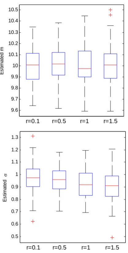
In this case study, we suppose n = 40. (AS will be shown, the bigger n is, the smaller estimation error is). For each case r∈ {0.1, 0.5, 1, 1.5}, the experiment is implemented 100 times and one of which is randomly selected to be illustrated. Therefore, total four of the four groups of 100 trials can be obtained, shown in Fig. 2. Correspondingly, Fig. 3 presents the box plot of estimations of the mean and deviation over the four groups of 100 trials.
6 8 10 12 14
0 1 O ber v at ions Ii (x )
r = 0.1 m = 10.0299 σ = 1.0011
x
(a)
6 8 10 12 140
0.2 0.4 E s ti m at ed di s tr ibut ion
6 8 10 12 14
0 0.2 0.4 0.6 0.8 1 1.2 1.4 O be rv a tions Ii (x )
r = 0.5 m = 10.1164 σ = 1.1437
x
(b)
6 8 10 12 140
0.05 0.1 0.15 0.2 0.25 0.3 0.35 E s tim ated di s tr ibu tion
6 8 10 12 14
0 0.2 0.4 0.6 0.8 1 1.2 1.4 Ob e rva tio n
s Ii
(x)
r = 1 m = 10.3136 σ = 1.1933
x
(c)
6 8 10 12 140
6 8 10 12 14
0 1
O
ber
v
a
tions
Ii
(x
)
r = 1.5 m = 10.0774 σ = 1.0019
x
(d)
6 8 10 12 140
0.2 0.4
E
s
timat
ed d
is
tr
ibut
[image:5.595.56.279.53.163.2]ion
Fig. 2 Estimated distributions of univiate normal with mean m = 10 and deviation σ= 1 in different cases: (a) r = 0.1, (b) r = 0.5, (c) r = 1, (d) r = 1.5.
9.6 9.7 9.8 9.9 10 10.1 10.2 10.3 10.4 10.5
r=0.1 r=0.5 r=1 r=1.5
E
s
tim
a
te
d
m
0.5 0.6 0.7 0.8 0.9 1 1.1 1.2 1.3
r=0.1 r=0.5 r=1 r=1.5
E
s
timated
[image:5.595.312.519.104.475.2]σ
Fig. 3 The estimated mean m and variance σin the cases r = 0.1, 0.5, 1 and 1.5 when n =40
As can be seen from Figs. 2 and 3, the estimated mean and deviation approach to the true ones when different length of interval observations can be obtained, and the estimated parameters becomes more accurate with decreasing of the width of the interval observations.
• Case 2) study
In this case study, we suppose r = 0.1. (AS can be seen from case 1) study, when r takes small value, the estimation result is more accurate.). For each case n ∈ {10, 20, 40}, the experiment is implemented 100 times. The estimation results
for mean and variance are presented in Fig. 4. From Fig. 4, we can see that, the larger the observation number n is, the estimation accurate is much higher.
9 9.2 9.4 9.6 9.8 10 10.2 10.4 10.6 10.8
n=10 n=20 n=40
Es
tim
a
te
d
m
0.5 1 1.5
n=10 n=20 n=40
E
s
tim
a
te
d
σ
Fig. 4 The estimated mean m and variance σin the cases n = 10, 20 and 40 when r = 0.1
From both the cases 1) and 2) studies, we can see that our proposed method can be used to estimate parameters involving interval-valued data, and we obtain the similar results as those done in the classical maximum likelihood estimation by using EM algorithm: the larger the observation number is, the the smaller the estimation error is, and the more precise the observations are, the smaller the estimation error is (i.e., the smaller the half bandwidth r is, the smaller the estimation accurate is).
V. CONCLUSIONS
[image:5.595.50.259.195.605.2]classical EM algorithm.
As an illustration, the proposed approach is used to estimate the mean and variance of univariate normal distribution. From the illustration result, we have reason to believe that it is possible to apply interval-valued EM algorithm to solve a wide range of statistical problems involving interval-valued data.
In further, it is interesting to apply the interval-valued EM algorithm to solve different problems involving interval- valued data, for instance, to estimate the regression coefficients of linear and nonlinear regression model involving interval-valued data, so as to establish regression model with crisp inputs and interval output, which is useful in engineering application where only interval values can be obtained for predicting a process parameter.
APPENDIX
Suppose the interval observation Ii(x) = [ai, bi] and the
p.d.f. g(x) with parameters ψ = (m, σ)', we have:
( )
(
)
( ) ( )( ) ( )
( ) ( ) ( )
(
,)
i i
i i
i i
xg x I x dx xg x I x dx
X I x
L I x
g x I x dx
=
∫
=∫
∫
Eψ
ψ (25)
where the denominator is given by (4). The numerator is
( ) ( ) ( )
( ) ( )
*2 *2
* *
exp exp
2 2
2
i
i
b i
a
i i
i i
xg x I x dx xg x dx
a b
m b a
σ π
=
⎡ ⎛ ⎞ ⎛ ⎞⎤ ⎛ ⎞
⎢ ⎜ ⎟ ⎜ ⎟⎥
= ⎢ ⎜− ⎟− ⎜− ⎟⎥+ ⎝⎜Φ − Φ ⎟⎠
⎝ ⎠ ⎝ ⎠
⎣ ⎦
∫
∫
(26)
where Φ(.) denotes the c.d.f. of the standard normal distribution, and x* denotes(x m− ) /σ for all x.
We finally compute
( ) ( ) ( ) ( ) ( )
( ) ( ) ( )
(
)
2 2
2
,
i i
i i
i i
x g x I x dx x g x I x dx
X I x
L I x
g x I x dx
⎛ ⎞ = =
⎜ ⎟
⎝ ⎠
∫
∫
∫
Eψ
ψ (27)
with
( ) ( ) ( )
(
) ( ) ( )
2 2
*2 *2
2
* *
*2 *2
* *
2 2 * *
exp exp
2 2
2
2 exp exp
2 2
2
i
i
b i
a
i i
i i
i i
i i
i i
x g x I x dx x g x dx
a b
a b
a b
m a b
m b a
σ π
σ π
σ
=
⎡ ⎛ ⎞ ⎛ ⎞⎤
⎢ ⎜ ⎟ ⎜ ⎟⎥
= − − −
⎜ ⎟ ⎜ ⎟
⎢ ⎝ ⎠ ⎝ ⎠⎥
⎣ ⎦
⎡ ⎛ ⎞ ⎛ ⎞⎤
⎢ ⎜ ⎟ ⎜ ⎟⎥
+ ⎜− ⎟− ⎜− ⎟
⎢ ⎝ ⎠ ⎝ ⎠⎥
⎣ ⎦
⎛ ⎞
+ + ⎜⎝Φ − Φ ⎟⎠
∫
∫
(28)
ACKNOWLEDGMENT
The authors are grateful to the contributions of Prof. Thierry Denoeux for our work.
REFERENCES
[1] H. Tanaka, “Fuzzy data analysis by possibilistic linear models,” Fuzzy
Sets and Systems, vol. 24, no. 3, pp. 363–375, Dec. 1987.
[2] P.Y. Hao, “Interval regression analysis using support vector networks,”
Fuzzy sets and systems, vol. 160, no. 17, pp. 2466-2485, Sep. 2009.
[3] M. Hladik and M. Cerny, “Interval regression by tolerance analysis approach,” Fuzzy sets and systems, vol. 193, pp. 85-107, Apr. 2012. [4] Y.-C. Hu, “Function-link nets with genetic algorithm based learning
for robust nonlinear interval regression analysis,” Neurocomputing, vol.72, no. 7-9, pp.1808-1816, Mar. 2009.
[5] C. Hwang, D.H. Hong, and K.H. Seok, “Support vector interval regression machine for crisp input and output data,” Fuzzy sets and
systems, vol. 157, no. 8, pp. 1114-1125, Apr. 2006.
[6] H. Ishibuchi and H. Tanaka, “Several formulations of interval regression analysis”. Proc. Sino-Japan Joint Meeting on Fuzzy Sets
and Systems, Beijing, China, 1990, pp. B2–2.
[7] J.-S. Jeng, C.-C. Chuang, and S.-F. Su, “Support vector interval regression networks for interval regression analysis,” Fuzzy sets and systems, vol.138, no. 2, pp. 283-300, Sep. 2003.
[8] M. Sato-llic, “Symbolic clustering with interval-valued data,” Procedia
Computer Science, vol. 6, pp. 358-263, 2011.
[9] T. Denoeux and M. Masson, “Multidimensional scaling of interval-valued dissimilarity data,” Pattern recognition letters, vol. 21, no.1, pp. 83-92, Jan. 2000.
[10] F. Palumbo and C.N. Lauro, “A PCA for interval-valued data based on midpoints and radii”. In: new developments in Psychometrics, H. Yanai, A. Okada, K. Shigemasu, Y. Kano and J. Meulman, Eds., Psychometric
Society, 2003, pp. 641-648.
[11] H. Wang, R. Guan, and J. Wu, “CIPCA: Complete-information- based principal component analysis for interval-valued data,”
Neurocomputing, vol. 86, pp.158-169, Jun. 2012.
[12] T. Denoeux, “Maximum likelihood from fuzzy data using the EM algorithm,” Fuzzy sets and systems, vol. 183, no. 1, pp. 72-91, Nov. 2011.
[13] T. Denoeux, “Maximum likelihood estimation from uncertain data in the belief function framework,” IEEE Transactions on knowledge and
data engineering, to be published.
[14] B. Quost and T. Denoeux, “Clustering fuzzy data using the fuzzy EM algorithm,” In: the 4th international conference on Scalable uncertainty
management, Toulouse, France, 2010, pp. 333-346.
[15] Z.-G. Su, P.-H. Wang, and Z.-L. Song, “Kernel based nonlinear fuzzy regression model”, Engineering applications of Artificial Intelligence, to be published.
[16] A.P. Dempster, N.M. Laird, and D.B. Rubin, “Maximum likelihood from incomplete data via the EM algorithm,” Journal of the Royal
![Fig. 1 Boxcar function I(x) for interval [a, b] containing x](https://thumb-us.123doks.com/thumbv2/123dok_us/1277789.656082/2.595.94.241.363.494/fig-boxcar-function-i-x-for-interval-containing.webp)