Two Area Load Frequency Control Using DE Tuned PID Controller with Nonlinearity

Two Area Load Frequency Control Using DE

Tuned PID Controller with Nonlinearity

Arti Sexana

_{, Kapil Parkh}

1, 2_{Electrical Engineering, SITE, Nathdwara}

Abstract: A coordinated operation of two or more than two power area is essential today for fulfilling the end consumers load demand for which this kind of structure in power system is termed as interconnected area. Their proper and successful operation requires minimal changes in the frequency and tie line power flow among their tie lines. Hence, keeping the frequency and tie line power flow close to constant is of key significance here. Normally, for a single area system load frequency control (LFC) is quite simple, but for such an interconnected area it is quite a task. Like in single area system too, the LFC in case of two area interconnected system can be bettered with the inclusion of controller. Therefore, PID controller is used in the presented work in LFC loop. Its performance could further be enhanced by the use of some optimization technique for which Differential Evolution (DE) algorithm has been put to use and it will help to reduce the time domain objective of the work. In the process of analysis the generation rate constraint (GRC) is also considered to account for the non linearity present in the interconnected system going closer to real practical scenarios.

For the LFC PID controller is used here with the optimization provided by DE (Differential Evolution) and BOFA (Bacteria Foraging Optimization). Later both these techniques were compared with each other and with conventional controller and with Genetic algorithm (GA) based controller. The simulation of the two area non reheat thermal interconnected system is carried out in MATLAB/SIMULINK under different cases. The cases falls under two category of saturation limit one with α=±0.05 and other with α=±0.025. The case are, 5% step change in load of both the areas, change in the system parameters by 50% (either increasing it or decreasing the particular parameter) and observing the settling time for deviation in frequency and tie line flow for both the areas. To evaluate the usefulness of the proposed method, we compare the answer of this method Differential Evolution (DE) with the Bacteria Foraging Optimization (BFOA) method of the PID controller technique for the same composite system. Investigations show that the proposed DE algorithm is superior to the BFOA technique. Simulation results show that the differential evolution-based tuning of the PID controller performs better than the BFOA optimization-based PID controller.

Keywords: Automatic Generation Control; Load Frequency Control; Generating Rate Constraint Differential Evolution; Bacteria Foraging Optimization

I. INTRODUCTION

A. Introduction

It is of utmost importance to safeguard the territory and keep the frequency close to the booked qualities, especially in large power plants with interconnected control area, load frequency. A well-defined performance framework should be able to achieve the satisfactory quality of the power supply by maintaining the frequency and voltage within the core as much as possible [4].

The system frequency is affected by changes in the network load, essentially the system frequency. However, reactive power is not significantly affected by frequency changes, but variations in voltage magnitude have a major impact on them. Consequently, there is an independent management of control in the energy system on the reactive and true power. Therefore, system frequency and active power are essentially controlled by load frequency control, while reactive power and voltage are essentially managed by a programmed voltage regulator.

A high quality power system must have controllers that maintain the superior performance despite the fact that the load varies randomly. The purpose of AGC in an interconnected system is to control frequency and power flow so that the system frequency is immune to interference [4].

B. Objective Function

For both the areas frequency deviation and tile line flow a performance index is defined using Integral of Time multiply Absolute Error (ITAE) of these two parameters. Objective function is,

J=∫ (|∆ | + |∆ | + |∆ | (1)

Hence the design problem of PID controller is stated as Minimize J subjected to

≤ ≤ , ≤ ≤ , ≤ ≤ (2)

II. SYSTEM MODEL

A. AGC in Two Area System (Thermal Thermal System without Heat Turbine)

Fig.1 shows two area interconnected by tie line & fig.2 shows The area 1 & area2 shows different parameters where f1 & f2 is the system frequency (Hz), R1 & R2 is the regulation constant (Hz/unit), TG1 & TG2 is the speed governor time constant (s), TT1 & TT2is the turbine time constant (s) ,TP1& TP2 is the power system time constant (s), ACE1& ACE2 is the area control error, ∆PD1 & ∆PD2is the load demand change, ∆PC1& ∆PC2 is the change in speed changer position, ∆PG1& ∆PG2 is the change in governor valve position, KP1 & KP2 is the power system gain, and ∆Ptie is the change in tie line power for area1 & area2 . In addition, nonlinear model shows

in fig.2 (with α = ±0.05 and α=±0.025) the linear model of a non-reheat turbine. This is to take into account the generating rate constraint (GRC), where PID controller represent by KP is proportional gain, KI is the integral gain, and KD is differentia l gain, respectively. The PID controllers in both areas were considered to be identical. The real power transfer between the tie line of two area system [5],

P =| | | | sinδ (3)

(X =X1+Xtie+X2, δ = δ1+ δ2)

Tie line flow changes by small amount ΔP = Δδ = PΔδ = P (Δδ − Δδ )

The below figure represents the system that has to be focused and examined here containinf PID as controller and two area non reheat thermal system.

Fig.2 Nonlinear Turbine Model with GRC [5]

III. DIFFERENTIAL EVOLUTION (DE) TUNED PID CONTROLLER

A. Proportional Integral Derivative Controller

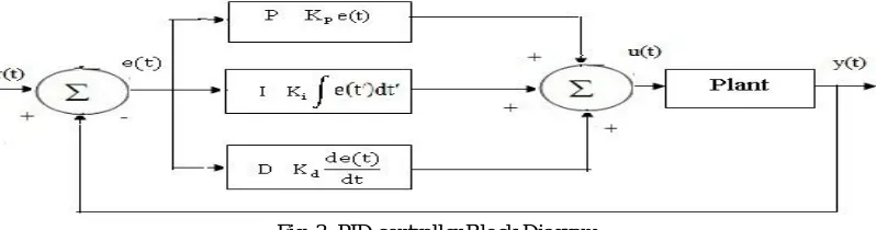
Fig. 3 shows PID controller block diagram. The output in the given controller depends upon the error signal e(t) generated by comparing the desired set point with the processed variable. The error is then corrected based on integral, proportional and derivative control that’s why it’s named as PID controller [21].

Fig. 3: PID controller Block Diagram

Fig.4 shows DE-tuned PID controller shows. The subject here is the parameters of the controller which should have a value close to or nearly equal to the best possible value i.e. optimal solution. There are namely three parameters Kp, Ki and Kd gain of PID controller

Fig. 4: DE Tuned PID Controller

B. DE Optimization Technique

Optimization is the process of getting the solution which is best applicable at a time. There are many ways; one of it is metaheuristic techniques that improve the given solution by iteration with respect to quality of measures. It uses no or very few assumption about the concerned problem and can search through large space of candidate solution. But it doesn’t ensure optimal solution[26].

One such technique falling under this category is Differential Evolution (DE). It utilizes real valued functions that are multidimensional. Although, it doesn’t involve gradient of the problem in optimization i.e. it doesn’t require problem to be differentiable as with the case in classical optimization. Therefore, optimizations of non continuous and noisy problem are possible through it.

It is a population based stochastic algorithm given by Storm and Price in 1996. The optimization problem can be stated as, Minimize f(X)

Where X=[x1, x2, x3,. . . ., xd], d= number of variables.

1) Process: DE is different from Evolution algorithm in the matter of application of mutation, as it is applied first to obtain the trial vector. Then, it is used within the crossover for the production of one offspring. Also, mutation steps are not sampled from the already known probability distribution function[26]. The DE algorithm is a population-based algorithm, similar to genetic algorithms that use similar operators. Crossover, mutation and selection. The main difference in creating better solutions lies in the fact that genetic algorithms rely on crossing, whereas DE relies on mutation operations. This main operation is based on the differences of pairs of solutions chosen at random in the population. The algorithm uses a mutation operation as a search mechanism and a selection operation to direct the search to the prospective regions of the search space. The DE algorithm also uses a non-uniform crossover, which allows child vector parameters to be taken more frequently by one parent than by others. By using the components of the existing population members to construct the test vectors, the recombination operator (crossover operator) effectively mixes information on successful combinations, thus enabling the search for a better solution space[6].

2) Algorithm

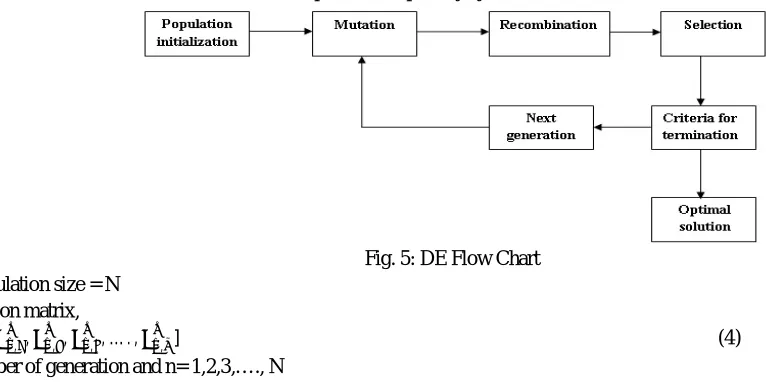
Fig.5 shows DE flow chart and defines different process adopted by system.

Fig. 5: DE Flow Chart Let population size = N

Population matrix,

, = [ , , , , , , … . , , ] (4)

g= number of generation and n= 1,2,3,…., N

a) Initial Population: The population at the initial point is generated between upper and lower bound.

, = , + ( )∗( , − ,) i= 1,2,3, . . . .D (5)

,= variable upper bound

,= variable lower bound

b) Mutation: Randomly three other vectors , and are chosen from each parameter vector.

= + ( − ) (6)

= donor vector F varies from 0 to 1.

c) Recombination: From donor and target vector i.e. _, and _, respectively a trial vector is developed _, .

, =

, ( )≤ =

, ( ) > ≠

(7)

= random number which is an integer [1, D] = recombination probability

d) Selection: The comparison of target vector is taken with trial vector and which ever has the lowest function value is selected for next population.

= , <

ℎ (8)

IV. RESULT ANALYSIS AND DISCUSSIONS

This result represents a benefit of the novel artificial intelligent search approach to discover the parameter optimization of the linear LFC taking into account the proportional integral derivative control (PID) for an two area non reheat system. A two-zone non-reheat system is contemplated to be equipped with a PID controller. The contrast of the bacterial foraging (BFOA) and differential evolution (DE) optimization algorithm is used to search for optimal control parameters to reduce the time domain objective function. The overall performance of the proposed approach was evaluated by the performance of the DE algorithm with the purpose of demonstrating the advanced performance of the proposed DE regulations in tuning the PID controller. In contrast to the BFOA PID method and DE PID, the effectiveness of the proposed DE PID over different running situations and device parameter variations is verified.

Table 1 shows PID parameters at different GRC & The two area thermal-thermal non reheat system tested with two nonlinearity as different GRC as α=±0.05& α=±0.025

Table 1: PID Parameter of when GRC α=±0.05 & α =0.025

S. N. PID

Parameter

With GRC α=±0.05 With GRC α=±0.025

BFOA PID Controller

DE PID Controller BFOA PID Controller DE PID Controller

1 KP 0.1317 0.4238 0.1317 0.3433

2 KI 0.41873 0.7649 0.41873 0.3385

3 KD 0.2506 0001 0.2506 .01000

A. Result of DE Optimized PID Controller

Fig.6 shows the best cost function with an iteration of DE algorithm and its definitely the best value gets by DE algorithm.

Fig.6: Convergence of objective function for gbest Load Frequency Control system at GRC α=±0.05 & α=±0.025

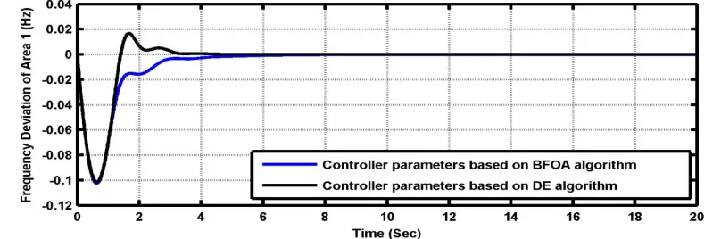
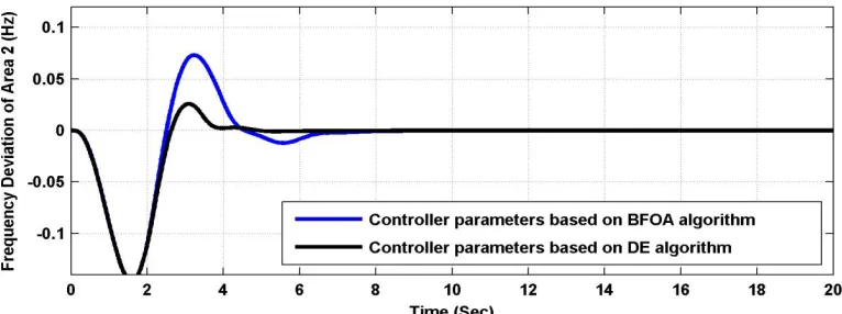
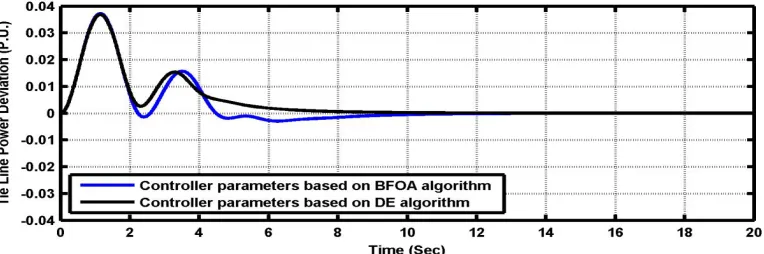
1) Case-1: 5% Step Increase in Demand of the Area-1 (∆PD1)

Fig. 7 to 9 shows frequency deviation of area-1, 2, tie line power deviation of 5% step load change in area-1 with α = ±0.05 & α =

±0.025. The system shows less settling times compared to modern optimization approaches BFOA optimized PID controllers.

Fig. 8: Frequency Deviation of Area-2 for 5% Step Load Change In Area-1 at α=±0.025

Fig. 9 Tie Line Power Deviation for 5% Step Load Change in Area-1 at α=±0.025

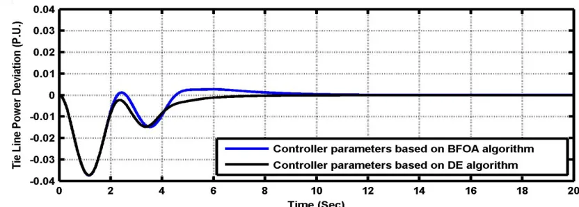
2) Case-2 :5 %Step Increase in demand of the area-2 (∆PD2)

Fig.10 to 12 shows response area1, 2, tie line power deviation .The proposed DE optimized PID controllers show best dynamic performance compared to BFOA optimized PID controllers. The DE PID controller is shown superior response than BFOA PID controller and system shows reduce settling time.

Fig. 10: Frequency Deviation of Area-1 for 5% Step Load Change In Area-2 at α=±0.05

Fig. 12: Tie Line Power Deviation for 5% Step Load Change in Area-2 at α=±0.025

3) Case-3 Effect of Parameter Variation on System Response

Fig.13 to fig, 16 shows response area1,2,tie line power deviation with a 50% increase, decrease in T12 & 50% increase, decrease in

Tg at α= ±0.005 & α= ±0.025 . It is obvious that the dynamic performance with proposed DE optimized PID controller is superior

to BFOA optimized PID controller Hence, it can be concluded that the proposed control approach provides a strong control under large changes in the system parameter variations.

Fig. 13: Frequency Deviation of Area-1 for 5% step change in area-1 with 50% Increase in T12 at α=±0.05

Fig. 14: Frequency Deviation of Area-2 for 5% step change in area-1 with 50% Decrease in T12 at α=±0.025

Fig. 16: Tie Line Power Deviation for 5% step change in area-1 with 50% Decrease in Tg at α=±0.025

Table 2: Performance Indices Different GRC at α=±0.005 & α=±0.025

S.N. Saturation Parameter change BFOA PID

Controller

DE PID Controller

1 Step increase in demand of the second area (∆PD1)

Area-1 at α=±0.05 4.3604 3.0630

Area-2 at α=±0.025 6.5512 3.7986

Strap line power deviation at

α=±0.025

9.3116 7.6439

2 Step increase in demand of the second area (∆PD2)

Area-1 α=±0.05 6.3275 3.1147

Area-2 at α=±0.025 7.4855 5.4959

Strap line power deviation at

α=±0.025

9.3121 7.6436

3 Effect of parameter variation on system response

By 50% T12 Increase at

α=±0.05

Unstable 0.5905

By 50% T12 Decrease at

α=±0.025

3.7706 3.1066

By 50% Tg Increase α=±0.05 Unstable 0.6793

By 50% Tg Decrease at

α=±0.025

2.4102 1.8270

V. CONCLUSIONS

REFERENCES

[1] Aravindan P, Sanavullah MY, “PID based automatic frequency control of two area power system with GRC”, Int J Comput Intell Res, 5(1), pp.37–44, 2011.

[2] D Sasi, P Jisha and Kuruvilla, “Modelling and simulation of SVPWM inverter fed permanent magnet brushless dc motor drive." International Journal of Advanced Research in Electrical, Electronics and Instrumentation Engineering 2, no. 5, pp. 1947-1955, 2013.

[3] Kundur P, “ Power system stability and control,” McGraw-Hill; 1994.

[4] Roy R, Bhatt P, Ghoshal SP, “ Evolutionary computation based three area automatic generation control”, Int J Electrical Power Energy System 37(8), pp. 5913–24, 2010.

[5] Khodabakhshian A, Hooshmand R, “A new PID controller design for automatic generation control of hydro power systems”, Int J Electrical Power Energy

System 32(5), pp. 375–82, 2010.

[6] Bhatt P, Ghoshal SP, Roy R, “ Load frequency stabilization by coordinated control of thyristor controlled phase shifters and superconducting magnetic energy

storage for three types of interconnected two area power systems”, Int J Electrical Power Energy System, 32(10), pp.1111–24, 2010.

[7] Atul Ikhe, Anant Kulkarni, Dr.Veeresh ,“Load Frequency Control Using PID Controller of Two Area -thermal Power System”, ISSN 2250-2459, Volume 2,

Issue 10, October 2016.

[8] MA Zamee, MM Hossain, A Ahmed and KK Islam, "Automatic generation control in a multi-area conventional and renewable energy based power system using differential evolution algorithm." In Informatics, Electronics and Vision (ICIEV), 2016 5th International Conference on, IEEE, pp. 262-267, 2016. [9] E Nikmanesh, O Hariri, H Shams and M. Fasihozaman, "Pareto design of load frequency control for interconnected power systems based on multi-objective

uniform diversity genetic algorithm (MUGA)," International Journal of Electrical Power & Energy Systems 80, pp. 333-346, 2016.

[10] RK Sahu, S Panda,A Biswal and GTC Sekhar, "Design and analysis of tilt integral derivative controller with filter for load frequency control of multi-area interconnected power systems," ISA transactions 61, pp. 251-264, 2016.

[11] S Kumari, G Shankar and Prince A, “Load Frequency Control Using Linear Quadratic Regulator and Differential Evolution Algorithm”, International