The fourier phase problem

~

thesis presented for the degree of

GDoctor of GJ>hilosophy

in G£1ectrical 'Engineering ,

in the

G(Jniversity of Canterbury,

Christchurch, New Zealand

by

W.R. Fright

B.Eu(Hons

0

ABSTRACT

Theoretical and practical aspects of solving the Fourier phase prob-'if y~

lem are presented.

Reconstructing an image, or the phase of its Fourier transform

(visibility), when only the ·magnitude, or intensity, of its visibility

is given, presents what is called a phase problem. If it is to be a

Four-ier phase problem, then samples of the visibility magnitude must be

avail-able at at least twice the Nyquist rate in each direction in Fourier space.

The phase reconstruction algorithms which are discussed in this thesis can

then be employed.

The fields of technical science in which Fourier phase problems arise

are listed and commented on. Particular attention is paid to

high-resolu-tion optical astronomy, and to a lesser extent to radio astronomy. Recent

advances in astronomical imaging techniques are discussed and illustrated

with results obtained from optical laboratory simulations. The phase

prob-lem associated with X-ray crystallography is also discussed and is shown

not to be a Fourier phase problem.

The question of uniqueness of the solution to the phase problem is

considered. Practical constraints that can be placed on real-world images

are shown to reduce the ambiguity of the solution, especially in more than

one dimension. The constraint of non-negative realness, or positivity, of

the image, is particularly restrictive. Existing theory on the uniqueness

question is reviewed. One-dimensional phase problems usually have

ambigu-ous solutions, whereas in two (or more) dimensions it appears that

solu-tions are almost always unique.

Some phase reconstruction algorithms that have proved effective in

practice are explained. Algorithms for solving one-dimensional phase

problems are nearly all direct, but additional information is usually

necessary to resolve the inherent ambiguity of the solution. Two- (or more)

dimensional algorithms, on the other hand, are nearly all iterative.

The practical implementation of a discrete two-dimensional phase

reconstruction algorithm is described. The algorithm, called crude phase

phase. A method of optimising the fidei.li ty of the estimated phase is

described which requires no a priori information about the image.

Further improvement of the estimated phase is obtained by iterative

processing of the kind pioneered by Fienup. Certain kinds of image are

identified as being difficult to reconstruct unless CPE and the iterative

algorithms are supplemented by ancillary procedures. Two such procedures

are described. The first, called pre-filtering, is designed to reduce

noise. Although CPE and the iterative algorithms are not unstable with

noisy data, the quality of the reconstruction is shown to be enhanced by

pre-filtering. The second ancillary procedure has two stages called

defogging and refogging. They are shown to assist in reconstructing

images which are comprised of faint detail superimposed on large amplitude

backgrounds. Defogging modifies the visibility magnitude before the

actual reconstruction algorithms are invoked. Fine detail in the image is

usually recovered more effectively in this way. In a range of situations

of potential practical importance, the detail is often impossible to

recover without the aid of the ancillary procedures.

CPE, the iterative algorithms and the ancillary procedures are

com-bined into a composite reconstruction scheme. Examples are presented

using both computer-generated data and data measured in the optical

labora-tory. The composite scheme is shown to be particularly useful for

TABLE OF CONTENTS

ABSTRACT

ACKNOWLEDGEMENTS

PREFACE

GLOSSARY

CHAPTER 1

1.1 1.2 1.3 1.4 1.5 1.6 1.7

CHAPTER 2

2.1

2.2

2.3

2.4

CHAPTER 3

3.1 3.2

PRELIMINARIES

The Fourier transform

The Phase Problem

The Far-field

Compact Images

Sampling

~be Discrete Fourier Transform

Autocorrelation

HOW SOME PH.~E PROBLEMS ARISE The Astronomical Setting

2.1.1 Resolution

2.1.2 The Seeing Problem

Astronomical Optical Interferometry

2.2.1 Speckle

2.2.2 Labeyrie

2.2.3 2.2.4 2.2.5 2.2.6 2.2.7 Deconvolution Holography Knox-Thompson

Speckle masking

Shift-and-add

Radio Astronomy

2.3.1 The VLA

2.3.2 Closure phase

X-ray Crystallography

UNIQUENESS

Phase Dominance

Image-form and how i t is Constrained

3.3 Uniqueness in One Dimension

3.4 Uniqueness in Two or More Dimensions

3.5 Another Uniqueness Argument 3.6 Effect of Noise

CHAPTER 4 PHASE RECONSTRUCTION ALGORITHMS 4.1 Algorithms for 1-D

4.1.1 Apodisa·tion

4.1:.2 Zero-matching

4.1.3 Special cases 4.2 Algorithms for 2-D

4.2.1 Gerchberg and Saxton

4.2.2 Fienup

4.2.3 Phase recovery using phase closure

4.2.4 Maximum entropy 4.2.5 Special cases

CHAPTER 5 BATES' ALGORITHM AND ITS PRACTICAL IMPLEMENTATION 5.1 Bates' l-~.lgorithm

5.2 Crude Phase Estimation 5.3 Centro-symmetric objects

CHAPTER 6 ANCILLARY PROCEDURES

6.1 Pre-filtering 6.2 Fog

6.3 Defogging 6.4 Refogging

I CHAPTER 7 A COMPOSITE PHASE RECONSTRUCTION PROCEDURE

-THE 1

CANTERBURY ALGORITHM 1

7.1 Strategy

7.1.1 Pre-processing

7.1.2 Defogging

7.1.3 Crude phase estimation

7 .1. 4 Starting the iterative algorithm

7.1.5 Iterative processing 7.1.6 Enlarging the image mask

7.1.7 Refogging

7.2 Reconstruction from Visibility Data Measured in the Optical Laboratory

7.3 Reconstruction of a Foggy Image 142

7.4 Reconstruction from ASI Data

Simulated in the Optical Laboratory 144

7.5 Reconstruction of an Extended Object 145

CHAPTER 8 FUTURE PROSPECTS AND CONCLUSIONS 153

8.1 Future Prospects 153

8.1.1 Fringe magnification 153

8.1.2 Improvements to CPE 154

8.1.3 New iterative algorithms 157

8.2 Conclusions 160

ACKNOWLEDGEMENTS

I deeply appreciate the guidance and encouragement my supervisor,

Professor R.H.T. Bates, has extended to me thoughout the course of this

research. His prodigious energy has been and will remain a source of

inspiration.

I am grateful for what I have learned from interacting with visiting

scientists, especially Dr G.J. Berzins of the Los Alamos Scientific

Labora-tory, Professor B.R. Hunt of the Digital Image Analysis LaboraLabora-tory, University

of Arizona, Professor M.V. Berry of the Physics Department, University of

Bristol, Dr J.R. Fienup of the Environmental Research Institute of Michigan,

and Dr P.J. Napier, deputy site manager of the United States National Radio

Astronomy Observatory's Very Large Array. I would also like to thank

Professor J.C. Dainty of the Physics Department, the Imperial College of

Science of Technology, for corresponding with Professor Bates and myself

on aspects of the CPE algorithm.

I thank Dr P.T. Gough, Dr R.M. Hodgson, Mr W.K. Kennedy and Mr P.L.

Squires of the Electrical and Electronic Engineering Department, University

of Canterbury, for their guidance during my time as both an undergraduate

and postgraduate student. The willing assistance provided by our

techni-cians, especially Colin Brittenden and Bob Young, and by all of the

Engineering Library staff is gratefully acknowledged.

Special thanks are due to my fellow research student Kathryn L.

Garden and to my old friend Dr Brent

s.

Robinson, now at the Biodynamics

Unit of the Mayo Clinic, not forgetting Don Baily, Dr Jason H.T. Bates,

Dr Phil Bones, Nigel Brieseman, Dr Pat Heffernan, Steve McNeill, Dr Rick

Millane, Robert Minard, Dr Andrew Seagar, Yeo Tat Soon and other members,

past and present, of our Biomedical Engineering group.

I wish to thank Drs Eric Hamilton, Richard Duke and Keith Turner

who gladly wrote for me during examinations. on this note, I would like to

go back eight years and thank Professor J.K. Bargh (now our Head of

Depart-ment), Mr A.H. Barth and Ms R.A. Ballin CBE for having the foresight and

confidence in me, to encourage me to begin engineering despite my then very

Warwick A. Norton and Giles H.T. Bates (while they were Professor

Bates' research assistants during several summers) provided me with their

capable assistance in the optical laboratory; Tim Densem, Geoff Graham

and Alex Joosten helped me both in and out of ~~e laboratory. To these

people I extend my sincere thanks.

During my thesis I benefited greatly from the practical experience

gained by working with Richard D. Jones of the Medical Physics and

Bio-engineering Department, Christchurch Hospital, Grant Carroll and Dr I.M.

Donaldson of the Neurology Department, Christchurch Hospital, and Dr A.E.

McKinnon, formerly computer manager at the Christchurch Clinical School of

Medicine, and now a systems analyst at Lincoln College, Canterbury.

I am a grateful recipient of a New Zealand University Grants Committee

Scholarship.

Finally, I give my deepest thanks to my parents and family, and to

my dear friends Sue Evans and Geoff Cron. I am indebted to Sue, not just

PREFACE

The work that is reported in this thesis began in 1980 when I

en-rolled for a Ph.D. I was following in the footsteps of several Ph.D

graduates who had worked on aspects of various phase problems with my

supervisor, Professor R.H.T. Bates. They had established an optical

laboratory for simulating the atmospheric seeing conditions that plague

high-resolution optical astronomy. They had developed new imaging

tech-niques such as speckle holography, speckle masking and shift-and-add.

Professor Bates suggested to me that we work together on developing

a more'global' approach to phase problems than had previously been

feas-ible. We decided to concentrate on problems of interest in radio

engineer-ing and optical astronomy, keepengineer-ing X-ray crystallography in mind in case

anything promising arose. As things have turned out, my results are

prob-ably of most immediate use in astronomical contexts, but they have very

much wider potential application.

As a lead in to my main research, and as a preliminary study of his

ideas on optical synthesis telescopes, Professor Bates encouraged me to

look at ways of amalgamating different one:-dimensional phase recovery

algorithms. One of Professor Bates• previous students, Dr P.J. Napier,

now deputy site manager of the United States National Radio Astronomy

Observatory's Very Large Array at Socorro, Ne>v Mexico, had explored the

use of complex zero theory in one dimension to solve phase problems of

interest in radio engineering. I took his results and applied them to the

data I had recorded in our optical laboratory, relating to simulations of

astronomical speckle interferometry with a long, thin pupil. The results

have been reported inapaper by Professor Bates and my.self to the Monthly

Notices of the Royal Astronomical Society.

In August 1981 Professor Bates hit on an idea for a direct method of

approximately solving the two-dimensional phase problem. I worked with him

and developed a practical phase recovery algorithm that is the centre-piece

of this thesis. Nore ex-periments were carried out in the optical

labora-tory, this time involving two-dimensional images. The experience gained

led to the development of ancillary procedures to assist the main phase

As my research progressed i t became clear to Professor Bates and myself that no one algorithm would ever be likely to be capable of

success-fully recovering phases under all conditions of practical interest. It

seemed essential to develop an armoury of algorithms and to combine them

into a composite procedure, capable of adapting to the requirements of

the wide range of data which can be expected in any practical application.

The 'Canterbury Algorithm' reported in this thesis is just such a procedure.

There is plenty of room for further improvement of course, and I am already

collaborating with several of Professor Bates' more recent research

stu-dents, trying to help them and attempting to refine my own ideas.

A chapter-by-chapter synopsis of the thesis now follows. I make

clear which parts of each chapter report my own original contributions. I

wrote the software for all of the algorithms and data reductions referred

to in this thesis.

The thesis is written in eight chapters. Chapter 1 introduces the

Fourier transform and related Fourier theory that underlies the phase

reconstruction algorithms described in later chapters. The reader is

intro-duced to the Fourier phase problem which is placed in context with other

kinds of phase problems.

In Chapter 2, the fields of astronomy and x-ray crystallography are

examined in some depth. High-resolution optical and radio astronomy are

of interest here because they present the kinds of phase problems that

are solvable by algorithms described in later chapters. X-ray

crystallo-graphy, on the other hand, is mentioned for quite. the opposite reason. It

is instructive to exruldne this application which presents a non-Fourier

type of phase problem as explained in §2.4.

Chapter 3 is a bridge between the first part of the thesis, which

introduces phase problems, and the latter parts which attempt to solve

them. This chapter seeks to answer questions like: is it the magnitude or

is i t the phase of the Fourier transform that is dominant in determining

the appearance of an image?; how is the ph~se of the Fourier transform

con-strained by the magnitude?; where and in what respects can the solution to

the Fourier phase problem be expected to be unique? Most of this chapter

is of course a review of previous researchers' results. Significant parts

of it are, however, 'Canterbury contributions', the refinements of

collab-orative theoretical specula·tions and detailed analysis by Professor Bates

Several of the known phase•reconstruction algorithms that have been

proven to be effective in practice are reviewed in Chapter 4.

One-dimen-sional and two-dimenOne-dimen-sional approaches are treated. Particular attention

is paid to iterative two-dimensional phase reconstruction schemes,

espec-ially those due to Dr J.R. Fienup of the Environmental Research Institute

of Michigan.

Professor Bates' direct two-dimensional phase reconstruction algorithm

and its practical implementation is described in detail in Chapter 5. This

implementation is due to myself. Examples are presented to illustrate the

kinds of reconstruction that are possible for a range of different objects.

Certain kinds of images are identified in Chapter 6 as being difficult

to reconstruct by any one algorithm alone. Two ancillary procedures and

their remedial action are described. The underlying ideas were generated

jointly by Professor Bates and myself. The development of the procedure

is due to me. This is a short chapter which simply explains how to apply

the ancillary procedures.

Chapter 7 is where the whole phase reconstruction story comes

togethe~ A strategy is described which combines the pre-processing stages

introduced in Chapter 6, the direct phase estimation algorithm of Chapter

5, and the iterative techniques of Chapter 4. Several examples are

pre-sented to show how this composite phase reconstruction scheme performs with

data both computer generated and recorded in the optical laboratory. While

the overall strategy was hammered out in many prolonged discussions which

I had with Professor Bates, all of the actual development was done by

my-self.

In Chapter 8 a number of promising avenues for future research are

suggested. A summary of the thesis and conclusions follow at the end of

this chapter.

This is a convenient place to make some remarks about the diagrams

found throughout the thesis. Four different kinds of computer generated

graphics are used, namely, one-dimensional line plots, contour graphs,

relief maps and grey-scale displays that have been photographed. Whenever

~~ image is presented it is always the complete array that held the image

in the computer which is displayed. The size of this array for all phase

the true image in any example is never larger than 32 x 32 pixels to ensure an oversampling factor of at least 2 (§1.7). Whenever the visibility

mag-nitude is presented it is always the centre one-half that is displayed, with

the origin in the middle. In other words, the FFT array is displayed at

twice the scale used for displaying images, but is truncated to occupy the

same sized picture.

The amplitude range on nearly all figures is normalised since

compara-tive and not absolute amplitudes are usually of interest.

Papers and presentations prepared during the course of this research

are listed below in order of preparation:

Bates R.H.T., Fright W.R., Cady F.H., Berzins G.L. "Speckle processing,

shift-and-add and compensating for instrument aberrations", originally

published in Proc. Advanced Institute on Transformations in Optical

Signal Processing (held in Seattle, Feb. 1982) ; also in

".Transforma-tions in Optical Signal Processing" eds. 1'7. T. Rhodes, J. R. Fienup and

B.E.A. Saleh, SPIE, Bellingham, W.A. (1983).

Bates R.H.T. and Fright W.R. 1982. "Towards imaging with a speckle-inter-ferometric optical synthesis telescope", Hon. Not. R. astr. Soc. 198,

1017-1031.

Fright W.R. and Hinard R.A. 1983. "Optical and digital image processing",

presented at the IPENZ Conference (1982), Proc. IPENZ.

Bates R.H.T., Hunt B.R., Robinson B.S., Fright W.R., Gough P.T. ''Aspects

of speckle interferometric imaging", in Proc. International Conference

on Electronic Image Processing, University of York, U.K. (July 1982),

IEE Conference Publication 214, 164-168.

Fright W.R. and Bates R.H.T. 1982. "Fourier phase problems are uniquely

solvable in more than one dimension: III: computational examples for

two dimensions:, Optik 62, No. 3, 219-230.

Bates J.H.T., Fright W.R., Millane R.P., Seagar A.D., McKinnon A.E., Bates

R.H.T., Bates, G.H.T. and Norton W.A. "Subtractive image restoration.

III: some pratical applicatio:t1s", Optik 62, No. 4, 333-346.

Hunt B .R., Fright W .R., Bates R.H .T. 1983. "Analysis of the

shift-and-add method for imaging through turbulent media", J. Opt. Soc. Am.

73, No. 3, 456-465.

Bates R.H.T. and Fright W.R. 1984. "Reconstructing images from their

Fourier intensities", Chapter 5 of "Advances in Computer Vision and

Image Processing, Vol I: Signal and Image Reconstruction from

Incom-plete Data: Theory and Applications", ed. T.S. Huang, JAI Press, in

press.

Bates J.H.T., Fright W.R. and Bates R.H.T. 1984. "Wiener filtering and

CLEANing in a general image processing context", Mon. Not. R. astr.

Soc., in press.

Bates R.H.T. and Fright W.R. 1984. "Two-dimensional phase restoration",

in "Applied Fourier Analysis", Cambridge University Press, for the

Australian Mathematical Society, in press.

Bates R.H.T., Fright W.R. and Norton W.A. 1983. "Phase restoration is

successful in the optical as well as the computational laboratory",

GLOSSARY

All mathematics and symbols are typed in italics. Symbols

represent-ing vector quantities are underlined. Where special terms are first

defined they are also typed in italics. The first time a symbol or an

abbreviation appears it is defined, but for reference the main ones are

defined below. Note that image space quantities and their Fourier

trans-forms are denoted by lower- and upper-case symbols respectively, unless

other symbols are more appropriate.

(i)

++

Jrx;

J

drJ( )

I I

phase{

*

f)

±

< >

u i

n

e

~

Re

Im

EVEN Symbols 1 J

a Fourier pair

K-dimensional integral

K-dimensional volume element

magnitude of a complex quantity

phase of a complex quantity

complex conjugate

convolution

correlation. The symbol representing a function is

repeated to represent the function's autocorrelation,

eg

ff

=

f

:k

f

time average, ie T

s (x_, t)

_{; J}

_s(x,t)

_dt

0

ensemble average, ie

<S (x)>

m

1 M

M

I

m=1

s (x)

m

union of sets identified by the subscript

i.

The subscript is omitted when there are only 2 sets, eg

{zm}

U

{zm*}

intersection of sets

member of the set

not a member of the set

real part of a complex quantity

imaginary part of a complex number

(ii)

ASI

CPE DFT

FT FFT

LHS

LO

LWH

MEM

OTF psf

RHS

rms

SAA

VLA

VLBI

Abbreviations

astronomical speckle interferometry

crude phase estimation

discrete Fourier transform

Fourier transform

fast Fourier transform

left hand side

local oscillator

Lynds, Worden, Harvey

maximum entropy method

optical transfer function

point spread function

right hand side

root-mean-square

shift-and-add

Very Large Array

Many activities in physics and engineering involve the determination

of one physical quantity from measurements of another. A relationship

between the quantities is formulated by considering the physics of the

situation and applying mathematical analysis. An effort is made to

express the relationship as a transformation which is inve~tible. In this

way it is possible to inverse transform the measurements to determine the

unknown quantity. This general description is familiar to anyone working

in astronomy, microscopy, radio engineering or crystallography. In these

fields, and others listed in Table 1.1, the transformation between

quan-tities is the

Fourier transform.

object

FT

~

visibility

FT

~

image

Figure 1.1. Diagram of Fourier transform (FT) relationships between

quantities.

In each field three quantities can be identified: They are often

given the names

object> visibility

and

imageJ

shown diagrammatically in

Figure 1.1. The name object is given to the physical quantity about

which information is being discovered. This is because the quantity is

often material, such as a star in astronomy or a microbe in microscopy.

The visibility, the quantity that is· often measured, or 'visible' as is

said in astronomical interferometry, is the Fourier transform of the

object. The inverse Fourier transform of the visibility called the

image. This is the inversion mentioned above. It is clear that the

'measurability' of the visibility affects the image obtained. It should

be noted that not all of the visibility can ever be measured. In addition,

the measuring instrument and environment may contain imperfections. In

an ideal situation, the image is a close facsimile of the object. Hence

form. In some applications the image can be partly measured. Also

there is often information available a priori to any measurement. All

this information can be incorporated into the calculation of the image.

Several schemes for doing this are discussed in Chapter 4. The

termin-ology of object, visibility and image is used throughout this thesis.

Alternative terms for the three quantities are listed in Table 1.1.

Table 1.1 Physical systems involving Fourier transforms.

Application

x-ray and neutron crystallography

microscopy

(acoustic, light and electron)

interferometry and spectroscopy

radio astronomical aperture synthesis

optical astronomical speckle imaging

radio engineering

ultrasonics

acoustics

communications

speech processing

Object

electron density of molecular structure

transmissivity or reflectivity of specimen (complex quantities in

general) "

spatially incoherent

radiating source distributions

coherently radia-ting or induced source distribu-tions

signal

1.1 THE FOURIER TRANSFOP~

Visibility

diffraction pattern

back focal plane field

interferometric visibility

spatial frequency spectrum far-field (Fraunhofer) radiating pattern temporal spectrum Image positive complex positive complex real

In this thesis an image and its visibility are described by complex

scalar functions, denoted by lower- and upper-case characters such as

f(~ and F(~~ where !£and ~are ]{-dimensional vectors in

image space

and

space.

The visibility is in general complex, so that i t possesses a magnitude and phase, both being functions of

u.

The magnitude

IF(u)

I

is called the

visibility magnitude

and the phase phase{F(~} is called the

visibility phase,

where

F(u)

=

IF(u)

I

exp(i phase{F(u)}

( 1.1)

i

is the imaginary operator=

/(-1).

The name

visibility intensity

is given to the quantity

2

IF(u)

I

=

F(u) F*(u)

(1. 2)

where

*

denotes the complex conjugate. When speaking qualitatively, the name visibility intensity is often used interchangeably with

visi-bility magnitude since the latter is related to the former simply by a

positive square root. The image too is in general complex, although

i t is ne9essarily real in many important physical situations, as is

indicated in Table 1.1, and is illustrated by the examples presented in

Chapter 2.

The Fourier transform is defined by (Papoulis 1962 p.7)

co

F(u)

=

J

(X)

f

f(g;;)

exp(-i2nu.!E) da(x)

( 1. 3)

-CO

where

frxJf

denotes a K-dimensional integral and

da()

is a volume element inK-dimensional space. f(x) and F(~ are called a Fourier transform pair

which is identified by

f(x) ++

F(u)

(1. 4)

The inverse Fourier transform is defined by

co

f(:E

=

f

(K)

J

F(~

exp(i2nu.?J_) da(u)

( 1. 5)

Almost all of the physical quantities studied here are either one

or two dimensional. In these cases the position vectors x and u are

expressed in Cartesian coordinates. This is the most convenient

coordi-nate system for the kinds of computations invoked in later chapters.

co (

F(u)

=

I

f(x)

exp(-i2~ux) dx

) -co

and in two dimensions is

co

F(u~v)

=

J J

f(x~y) exp(-i2~(ux

+

vy))

dx

dy

_co

1.2 THE PHASE PROBLEM

( 1. 6)

( 1. 7)

It is a simple matter to reconstruct the image from the visibility,

using (1.5), when both the visibility magnitude and visibility phase are

known. The image thus formed is called the

true image.

An effort to compute the true image, when the visibility magnitude is given accurately,

but the visibility phase is given only partially or not at all, presents

what is called a

phase problem.

This definition covers a broad range of problems. Each type of problem may require a different procedure for

its solution. It is therefore useful to attempt to classify phase

problems.

To begin with, phase problems can be said to be either imposed or

inherent. In the former case, information is typically to be transmi t·ted

over a channel, or stored in some way. For the sake of storage efficiency

the visibility phase may be represented only partially, or not represented

at all. After receiving or retrieving the stored information, a phase

problem arises vlhen reconstructing the image. Procedures to solve this

type of phase problem are of interest in the fields of speech processing

(Nawab 1982) and image processing (Devaney, Gonsalves and Chidlaw 1977).

Inherent phase problems occur when an object is to be sensed.

Sens-ing involves either, or both, the detection of wave motion, or the formSens-ing

of an image from the wave motion. The measurements of wave motion

corre-spond to the visibility. Visibility phase may then be a problem for one

or more of sevey-al reasons, depending on the application. When detectinq

wave motion, the accuracy of phase measurements decreases with increasing

frequency of wave motion. At frequencies below, say, 10 MHz, the

measure-ment of phase is not difficult. At frequencies higher than this, however,

difficulties can arise in maintaining stable phase references, as occurs

in Very Long Baseline Interferometry (VLBI) (§2.3). In the main this is

due to instrument imperfections causing increasing amounts of phase

higher, it is impossible to directly measure the visibility phase, and

the best that can be done is to store the phase implicitly in some sort

of hologram. With light, however, i t is possible to form an image, and

avoid the problems of measuring the visibility. When wave motion has

to propagate through a distorting medium however, a phase problem

definitely arises. This is the difficulty in optical astronomy (§2.2)

and to a certain degree in radio astronomy, (§2.3), where the distorting

medium is the earth's atmosphere (§2.1.2) . . In electron microscopy, only

intensities can be measured, but in both visibility and image spaces

(Missell 1978). In X-ray crystallography, only the intensity in

visi-bility space can be measured (§2.4).

The causes of phase problems can be summarised as being:

- deliberate reduction of phase data for increased transmission

or storage efficiency,

- insensitivity of receivers to the phase of high frequency

wave motion,

- distortion of the phase of wave motion during propagation, or,

- distortion of the phase of wave motion due to instrument

imperfection.

It is useful to further divide all phase problems into two types.

(i) The

pure phase problem

is posed as: reconstruct ~~e true image, given only the accurate visibility intensity. Certain characteristics of ~~e

true image are irretrievably lost when solving a pure phase problem, but

the appearance, or form, of the true image can still be recovered. This

is discussed further in Chapter 3. (ii) The

partial phase problem

is posed as: reconstruct the true image, given the accurate visibility

intensity, and partial measurements of either, or both, the visibility

phase or the image.

The phase problem in X-ray crystallography, and any type of

inten-sity interferometry, is unarguably a pure phase problem. All of the other

phase problems mentioned above are most often partial phase problems. In

radio astronomy (§2.3), and radio engineering (Jordan and Balmain 1968),

phase measurements are usually feasible. In optical astronomy, extensions

to speckle interferometry (§§2.2.4-2.2.7) are gaining increasing popularity

for obtaining phase measurements. In electron microscopy, the intensity

of the image is partly measured. The imposed phase problems, mentioned

reconstruc-tion from 'Fourier amplitude' problem (van Hove 1982).

The more difficult, and therefore more interesting phase problem is

the pure phase problem. Procedures for solving the pure phase problem

can only be simplified when used to solve the partial phase problem.

This thesis is concerned mainly with procedures for solving the pure

phase problem, in a general context, ie given IF(~

I,

find the form of

f(x),

with one caveati sufficient measurement must be made of the visi-bility intensity, for Fourier transform techniques to be applied. When

this is so, the phase problem is called the

Fourier phase problem.

This

condition is discussed quantitatively in §§1.5-1.7. X-ray crystallography

presents a phase problem where this condition is not met, as is explained

in §2.4. Solutions to the crystallographic phase problem, and other

non-Fourier phase problems, are not treated in this thesis. Table 1.2

summarises the above discussion on causes ru,d types of phase problems.

Table 1.2 Causes and types of phase problems

Application

X-ray and neutron crystallography

electron microscopy

radio astronomical aperture synthesis

optical astronomical speckle interferometrJ

optical astronomical speckle imaging

radio engineering

ultrasonics

acoustics

communications

speech processing

Causes

wavelength too short for sensing

wavelength too short for sensing

instrument imperfections

turbulent medium

instrument instability

turbulent medium

turbulent medium

accuracy depends on wavelength

distorting medium

deliberate _-), , optimisation

Type

pure, but non-Fourier

partial partial pure partial partial partial

[image:24.595.83.519.375.780.2]

1~3 THE FAR-FIELD

Many of the examples of phase problems examined in Chapter 2

involve

wave motion,

such as ultrasonic waves, radio waves, light waves or electron waves. In these cases the Fourier transform relationship

between the object and visibility can be derived by considering the

underlying physics of wave propagation. The derivation can be found

in a number of works dealing with subjects like optics (Born and Wolf

1976 Chapter 8, Goodman 1968 Chapter 4) or antenna theory (Silver 1965 §6.2). The latter stages of such derivations, showing the Fourier

trans-form as the limiting case of the Fresnel transtrans-form, are summarised below

for later reference.

Consider a region containing sources of wave motion, called the

source region,

embedded in homogeneous free space. P is an arbitrary

point within this region, which is shown shaded in Figure 1.2.

The source region is finite in size, or

extent,

and is described as

being

localised.

Cartesian coordinates (x~y~z) are set up in this space, with the origin chosen arbitrarily to be within the source region.

Figure 1.2 Coordinate systems for wave motion radiating from a localised

arbitrary point within the source region, which is shown

shaded.

Any planes, or lines, for which

z

is a constant, are described as being

transverse.

The largest transverse dimension of the source region is denoted by

D.

Wave motion radiating from the source region is des-cribed by the scalar linear wave function W(x~y~z~t). Suppose that this

wave motion is band-limited, and that the wavenumber k, wavelength

A,

and wave propagation speed a are related at a pa~·ticular angular frequency

k

=

2'1T/A ::::: W/c ( 1. 8)

It is convenient to have special notation for the wave motion in two

transverse planes. Firstly, the

equivalent source plane

is defined as a plane positioned at

z=zo,

such that all of the source region lies in the half space defined by

z

<

zo

(1. 9)

The wave function ~o(xoJYo₃t) is used to describe wave motion in the equivalent source plane, ,,vhere the arbitrary point

(xo

3

yo)

is called the

equivalent source point.

~o(xoJYoJt) is called the

equivalent source

distribution,

and corresponds to the object. Hence the name

object

plane

can be used for the equivalent source plane. Secondly, the

observation plane

is defined as a plane separated from the equivalent source plane by a positive distance z 1 • The '"ave function ~ 1 (x 111 y 1 J t)

is used to describe wave motion in the observation plane, where the

arbitrary point

(xl>Yl)

is called the

observation point.

lPl(XlJYl_,t) is conveniently referred to as the

diffracted field.

Now imagine

equivalent surface sources, or

secondary

sot~ces, placed on the

yo)

plane. Huygens' principle as expressed throug-h Green's theorems (Silver

1965 §4.1), confirms that equivalent sources can be chosen such that

the wave motion radiated from the equivalent sources is identical, for

z

>

zo,

to that radiated from the source region. The exact expressions

for the densities of the equivalent sources involve both ~o(xoJYo>t)

and its normal derivative (Silver 1965 §4.1).

The diffracted field corresponds to the visibility, which is the

quantity to be observed. It is impossible in practice to make

obser-vations over an entire plane. So it makes sense to restrict the

observation point to be within a circle, called the

obsel'Vat'ion cirele,

of diameter D1, ie

2

" D12!'4

X'l

+

y 1 ~ < ( 1.10)

This limits the resolution with which the equivalent source distribution

can be imaged. Further, the image formed or computed, in any practical

instrument, is limited to a finite area in image space, called the

field

of view.

Since the source region is localised, rays from all points

P

a finite part of the equivalent source plane. This finite region is

called the

equivalent source region,

and has a maximum transverse dimension denoted by

Do.

Because D1 is usually different to

D,

i t is clear that

Do

changes the further removed the equivalent source plane is from the source

region. It is usual, therefore, to choose

zo

to be the least value of z to satisfy (1.9). Hence for

D

1 fixed, and Zl large enough, i t follows

that

Do ::! D (1.11)

When

z

1 is sufficiently large compared with D 2

/A,

the density at an

equivalent source point (xo~Yo) becomes effectively proportional to

~(x₀,y₀~z₀, t) (Silver 1965 §4.6), provided (1.9) and (1.10) still hold.

In a practical instrument, the observation circle corresponds to the

aperture

or

pupil.

Hence the observation plane can be called the

aperture

plane

or

pupil plane.

As an example of the use of equivalent sources, consider how they

arise in astronomy. The actual sources are stars, which, as well as being

three dimensional themselves, are at different distances from the earth.

Nevertheless, all stars are represented by two dimensional sources on one

celestial sphere

of very large radius centred on the earth. Stars are then conveniently described in terms of their angular extent and

separa-2

tion. Because

z

1 is extremely large, in this case, compared with D

/A,

angular coordinates are effectively equivalent to Cartesian coordinates,

over the field of view.

The relationship between the diffracted field and the equivalent

source distribution can now be examined. To begin with, consider a

spatially coherent

source, for which the time dependence of ~(x,y,z~t) is, for all points

(x,y,z) monochromatic

of the wave function can be written as

\j!(x,y~z~t)

=\j!(x,y_,z) e:x:p(iwt)

The functional dependence

( 1.12)

The harmonic time dependence is omitted from equations involving

mono-chromatic wave functions, and is to be 'understood'. From scalar

diffrac-tion theory, the exact reladiffrac-tionship between ~o(xo,yo) and \j!l(Xl~Yl) is

(xo.,yo)

exp(ikr) oos(z.,r)

I

r dxo dyo

(1.13)

where ~is the vector shown in Figure 1.2 with magnitude r and oos(~£)

is the cosine of the angle between r and the z axis. If r is small, and

similar in magnitude to

D,

then no useful approximations can be made to (1.13). However in many situations r is much greater than Do~ D1 and

A.

It is then feasible to make approximations to terms involving r in {1.13).

If the largest angle between r and the z axis is never greater than

8°, say, then no more than l% error is incurred by replacing cos(~£) by unity, and similarly by replacing the

1/r

term by

1/zl.

The

exp(ikr)

term in (1.13) oscillates with period 2u. Because k may be very large,

the errors in a simple approximation to r may be multiplied up to be a

sizeable fraction of 2rr. The exact expression for r is

r (1.14)

which is conveniently expanded using the Binomial theorem. A useful

approximation to r is obtained by discarding terms in the expansion that

are higher than first order, and so

{1.15)

The simplified form of (1.13) that the substitution of (1.15) allows is

called the

Fresnel transform

or

F1•esneZ approximation,

and is written as (Goodman 1968 p.60)

(L 16)

The range of r over which this approximation is useful defines what is

called the

near field.

When r is large enough that quadratic terms in (1.16) can be discarded, and sufficient accuracy maintained, the

the

Fraunhofer

approximatio~ which is written as (Goodman 1968 p.6l)

co

J

f

lJ;o(xo.,yo) exp(-i2rr(xoxl + yoy1J

I

O.z1)) dxo dyo

-co

( 1.17)

-The point of transition from the near- into the far-field is gradual,

but can be quantified as follows. At an observation point (x₁_,y₁) , the

maximum differenced in wavelengths between paths from all points (x

0_,y0)_,

is given approximately by

( 1.18)

If

d

=

A/16

is considered to be a small deviation from a plane wave, then the near- and far-field are delineated by (Jordan and Balmain 1968

p.498)

( 1.19)

The relationship between the Fraunhofer approximation and the

Fourier transform is made evi_dent by the following approach. The

equiva-lent source distribution is confined to a finite region of the equivaequiva-lent

source plane. However, a function that is piecewise continuous across

the entire (x0_,y0 ) plane is given by (Silver 1965 §6.3)

-'

( l . 20)

Now f(xo.,yo) may be represented by the Fourier integral

co

f(xo.,yo)

=

JJ

F(x1.,y1J exp(i2rr(xoxl+ YoY1)) dx1 dy1 (1.21) -CO

Let the vector~ have components (Xl.,yl_,/(1- x12 - y12) ) , and the vector

r have components (x₀_,y0_,z). The complex exponential function

exp(i2rr(xox 1 + yoy1JJ may then be thought of as the distribution across the plane z = 0 of a plane wave with unit amplitude travelling in the

exp (i21T q.

( 1. 22)

z=O

Therefore, (1.21) is the superposition of many plane waves with amplitudes

F(x1.,y1).

Hence the name

anguZar speatrum of plane waves

(Booker and Clemmow 1950) is often given to the function F(x₁~y ₁), as expressed by

F(x1.,y1J

=If

f(xo.,yo) exp(-i2Tr(xoxl

+

yoy1JJ dxo dyo

( 1. 23) -00

Inspection of the right hand side (RHS) of (1.17) and (1.23) shows that

the Fraunhofer approximation is essentially a Fourier transform, with

some scaling of coordinates and a constant phase factor. Hence the

far-field diffraction pattern, for a monochromatic source, is the

Fourier transform of the equivalent source distribution.

Now consider a source that is

spatially inaoherent.

This means that the phase difference between the wave motion at any two points in the

source region varies randomly with time. Under these conditions, the

time variations of the equivalent source distribution are no longer of

interest. Instead, it is the distribution of intensity in the equivalent

source plane that is sought. The relative phases of the components in

the angular spectrum of the equivalent source distribution are randomly

distri~uted. Therefore, the wave motion must have a finite bandv1idth,

denoted in wavelengths by

6A.

If

6A

is small compared with the mean

wavelength

A,

ie

A./6A.

»

1 (1.24)

then the wave motion is called

quasi-monoahromatia.

The wave function ~(x.,y.,z) now represents the intensity of the wave motion in the band of

width 61.. centered at A.. The visibility is the Fourier transform of the

intensity distribution in the equivalent source plane (Goodman 1968

p. 106 ff). Hence the is also a.YJ. intensity distr:Lbution. The

is therefore real and non-negative when the source is spatially

1.4 COMPACT IMAGES

All real-world images are of finite extent. The size of the object

may be small enough to be within the field of view of the instrument. vJhen

the object is larger, however, the is truncated, because the field

of view is finite in any practical instrument. In either case, the

recorded image

f(x)

is inevitably contaminated by noise. The amplitude

and phase of the noise is assumed to be randomly distributed, with

root-mean-square (rms) amplitude denoted by the positive real number E. It

is pointless to worry about the amplitude of the image in regions where

If(~

I

~ E. Therefore the values of

x

for which

lf(x)

I

> s defines what is called the

support

off(~. It is useful to define an

image box

which has sides parallel to the Cartesian axes and which is just large

enough to encompass the support of the image. The image box of the image

f(x)

is denoted by

B(f),

and has a kth side of length

Lk(f).

The term

extent

is used to denote the size of the image box, ie the linear dimen-sions of the image.

If

f(x)

is of finite extent and contains no infinities, which is true

for all real world images, ie

lf(x)

I

<co_, for

xeB(fJ

(1.25)

then

f(x)

is called

compact.

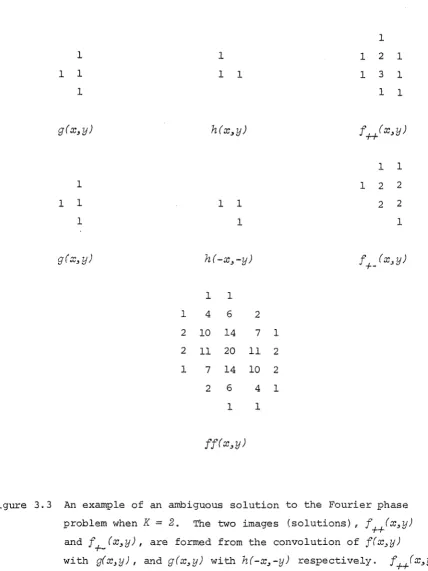
An example for is shown in Figure 1.3 .

y

Figure 1. 3

•

•

_r---:----1

1

I

t I

•

I .

I

L

₂

I

!L ______

..

-

L

_I

1. 5 SAMPLING

A compact image f(~ can be represented within B(f) to any desired

degree of accuracy by a trigonometric

Fourier series,

referred to here-after simply as a Fourier series. However, the Fourier series, if

permitted, reproduces f(x) periodically in adjacent image boxes

through-out all of image space. The periodic version of f(~ is denoted by p(x)

and has a Fourier series representation which is written as

where

p(~

=

K

1

I

V(f) k=l

m =-M k k

f(x)

=

p(~ _, x

e

B(fJ

F

are complex constants given by mt,_,_,mK

co

=

f

(K)

J

and

V(f)

is the volume of the image box, defined as

V(f)

=

J

(KJ

J

1

da(x)

B(f)

(1. 26)

(1.27)

(1.28)

( 1. 29)

The

Mk

are chosen in practice to be large enough so that f(~) is

repre-sented to the acc~racy limit set by the noise. The significance in

Fourier space, of the Fourier series in image space, is revealed by

substituting (1.28) into (1.3), thus

K

P(u)

=

I

k=1

( 1. 30)

where oK() is a K-dimensional delt.a function. This equation shows that

Positions of the delta functions in (1.30) define the set of sample points. The samples must be spaced in the kth dimension by aA, where

(1. 31)

which is known as the Whitaker, Shannon, or Nyquist rate (Bracewell 1978 Chapter 10). F(u) is said to be over-sampled when the sample points are spaced more finely than at the Nyquist rate, ie with spacing a~k' where

( 1. 32)

The effect in image space is to surround the image symmetrically

with empty space, which is called packing with zeros. The new image box size, B ... (f) , is larger than B (f) in proportion to the overs amp ling, ie

( 1. 33)

A single version of f(~ can be recovered from p(~) by multiplying by an appropriate window wd(~, thus

f(~ = p(~ wd(::c) ( 1. 34)

When F(u) is sampled at the Nyquist rate, the only possible choice of

wd( x) is the K-dimensional rectangular function rectK6~-/Li(f) ) )yt_{3JLK( f)))}

defined by

K

reatK(xlJ::c2 J.n xK) = TI rect(xkjL

1

~(f)) (1.35)

k=1

where (Bracewell 1978 p.52)

reat(::c) = 1 )

I

x

I

<

fz

(=

fz

)

lxl

= f§)

=

0 )

lxl

>

fz

The shape of wd(::c) can be 'relaxed' when Ffu} is over-sampled. That is, providing wd( x) is unity within B (f) , and zero outside of B ~ (f) , then it

can take any smooth form in between.

the

sampZing function sp(u)

is introduced, where

sp(J:!} ++ wd(x) ( 1. 36)

It is now convenient to define the

convolution

of two functions, f(~) and g(x), by

00

J

(KJ

J

f(~g(!!!_- ~

do(s)

(1. 37)

-CO

which is identified by

f(x) 0 g(~ ( 1. 38)

On defining G(u) and P(u) by G(u) ++ g(x) and P(J:!} ++ p(!!!), i t follows from substitution of (1.37) into (1.3) that

F(u) G(u) ++ f(~ fJ g(x) ( 1. 39)

which is known as the

convolution theorem

(Bracewell 1978 p.l08). There-fore,

fJ sp(u)

=

F(u} ( 1. 40)

which is the well known

sampling

theorem

(Bracewell 1978 Chapter 10). In the case of wd( uJ)

=

rectK(!!!) , sp (u) sincK( u) , t.vhich is a K-dimensional sine function (Bracewell 1978 p.62), defined by

K

( l. 41)

where

sinc(u)

=

(sin(nu))/ nu

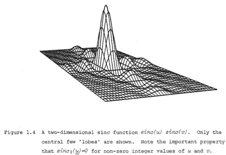
(1.42)

The one-dimensional sine function is zero for non-zero integer arguments.

The K-dimensional sine function is the product of K one-dimensional si,nc

Oth column. This important property of sincK(~ is useful in later

chap-ters for explaining uniqueness of phase solutions (§3.5).

Figure 1.4 A two-dimensional sine function

sinc(u) sino{v).

Only the central few 1 _lobes 1 _{are shown. Note t.l)e important property}

that sinc2{~=0 for non-zero integer values of

u

and

v.

1.6 THE DISCRETE FOURIER TRANSFORM

In §1.5 it is shown that a compact image can be reconstructed, albeit

periodically repeated, when only samples of the visibility are given.

Similarly, if the visibility is band-limited and is permitted to be

peri-iodically repeated throughout all of visibility space then the visibility

can be reconstructed given only samples of the image. The special Fourier

transform relationship dealing with only samples of both the visibility

and the image is called the

discrete Fourier transform

(DFT) (Stanley 1975 Chapter 9) . The DFT is defined in one dimension by

N

Fm

=

I

fn exp(-i2mnn/N)

(1.43)

n=1

where

F

=

F(m/N)

and

f

=

f(n/N)

so that

N,

which is both the number of

m n

visibility samples and the number of image samples, serves to define the

[image:35.595.67.514.140.446.2]

N

f

= (

1/N)

I

m

n=l

exp( i2rrmn/NJ ( 1. 44)

where

1/N

is necessa:ry to retain the correct amplitude of the image. The extension to K-dimensions is straightforward (cf (1.26)).

The advantage of the DFT is that i t allows data to be Fourier

trans-formed by a digital computer. However the computation time grows as N2

with the number of samples N if the DFT is implemented as a direct

algorithmi.c translation of (1.43) and (1.44), thereby tending to be

impracticably slow, especially when evaluating two-dimensio.nal

trans-forms. A modified algorithmic form of the DFT called the

jast Fourier

transform

(FFT) (Brigham 1974) is more useful since the computation time grows as only

NZog

2

N.

The FFT is used extensively in the sorts of

phase reconstruction algorithms that are described in Chapter 4.

1.7 AUTOCORRELATION

Measurement of only the intensity of the visibility is equivalent in

image space to measuring ~~e

autocorrelation

of the image. That is, the visibility intensity as defined in (1.2) is a Fourier transform

the autocorrelation function

ff(x).

In symbols,

IF

(u)

12

=

F*(u) F(u)

+--+

ff(x)

( 1.45)

which is known as the

autocorrelation theorem

(Bracewell 1978 p.llS), where

ff(x)

=

f

(K)

J

f(!!) f(x +!!) da(s) ( 1. 46)

_co

Autocorrelation is identified by

ff( x)

=

f(!!})

±

f(

iEJ

(1.47)

with

Autocorrelation is a specific case of

correlation

(Papoulis 1962 p.244) between two functions,

f(x)

and

g(x),

defined by

f(f!})

*

g(F£)

=

f

(K)

I

f(!!) g

+

x) da(s) ( 1. 48)

-CO

Inspection of the integral in (1.48) confirms that, if f(x) and g(F£)

extent of f(!E)

;k

g(x)

can be no greater than the sum of the extents of

f(x)

andg(!E), ie

(1.49)

( 1. 50)

The support of

ff(x)

is a convex figure just fitting inside

B(ff),

which is called the

autoaorreZation box.

From the sampling theorem (§1.5), the samples of jF(~

!

2 must be spaced, in the kth dimension, by

~\, where

( 1. 51)

Comparison of (1.31) ,with (1.51) confirms that samples of visibility

intensity must be spaced by at least twice the Nyquist rate.

A real function that has both positive and negative parts is called

bipoZar;

a real and non-negative function is called

positive.

Restric-tions that are placed on the visibility, and on the autocorrelation, for

complex, bipolar and positive images, are summarised in Table 1.3. Note

that a function F(~ is called

aonjugate symmetria

when

F(-u)

=

(u) (1.52)

and is called

aentro-symmetric

when

Table 1.3 Restrictions on the visibility and on the autocorrelation.

complex bipolar positive

';) ~ \

F(u)

complex complex complex

conjugate conjugate symmetric symmetric

jF(!£}!2

positive positive positive

centro-

centro-symmetric symmetric

ff(!E) complex bipolar positive

·conjugate centro-

CHAPTER 2

HOW SOME PHASE PROBLEMS ARISE

In this chapter, representative examples are given of physical systems

in which phase problems arise. Two types of examples are given. Firstly,

there are those phase problems which satisfy the definition of a Fourier

phase problem (§1.2). Possibly the most topical of these is the phase

problem encountered in astronomy. This is the sort of problem that is

solvable by the procedures introduced in this thesis. That is why many of

the objects used in examples given in later chapters have the appearance

of space objects. Sections 2.1 to 2.3 deal with the branch of astronomy

which is concerned with imaging stellar objects. The 'astronomical scene'

is set in §2.1. Then the principle of interferometry is discussed- a

principle shared in common by radio astronomy and high resolution optical

astronomy. It is usual to think of interferometry as involving the

reception of signals by separated telescopes or antennas. However, the

same process occurs in a single large aperture telescope, ie an

inter-ference pattern is produced. By appropriately processing the interference

information the size of a typical stellar object can be determined. \vith

some procedures, only the autocorrelation of the image is formed. With

other procedures, an estimate of the true image is formed. This depends

on how much phase information can be recovered. Just what can be achieved

in optical and radio astronomy is discussed respectively in §§2.2 and 2.3.

Secondly, there are those types of phase problems which do not satisfy

the definition of the Fourier phase problem given in §1.2. A specific

example of this second type of problem, which is outlined in §2.4, is the

phase problem encountered in X-ray crystallography. The physics behind

the use of the Fourier transform in crystallography is explained first.

From there it is shown why the phase problem for objects which are

repeti-tive structures, such as crystals, is not directly solvable by the

proce-dures with which this thesis is mainly concerned.

2.1 THE ~STRONOMICAL SETTING

The objects of interest in astronomy are planets and moons, the sun,

stars, nebulae, galaxies and other celestial objects. The first two are

either case, the sources of the wave motion are almost always

incoherent. Consequently, the kinds of astronomical images which are of

interest here are positive (§1.3). The majority of observations of these

phenomena involve wave motion at the wavelengths of visible light, infra

red, radio waves and X-rays. Because the objects are removed from the

earth by enormous distances, then at any of the above wavelengths a

Fourier transform relationship holds between the object and the wave motion

incident on the earth (§1.3). At a distance of less than lOkm from the

earth, which is miniscule relative to the distance the wave motion must

travel, is the earth's atmosphere (Figure 2.1). The density of water

vapour and gases in the atmosphere varies continuously, mainly because of

temperature fluctuations (Roddier 1981) . This means that the refractive

index of the atmosphere varies, and wave motion is distorted as it

propa-gates through. In turn this gives rise to what is known as a

problem

for ~bvious reasons. Detailed descriptions of the atmospheric seeing problem are found in the following articles and in the references

quoted therein: Bates 1982b, 1983, Dainty 1975, 1982.

light

years

-10 kmi

\

\

\ I

Spatially incoherent

radiating or reflecting

celestial

object.

Turbulent atmosphere.

Telescope:

_ _ _ _

...,'~-'

_ _

.:.:.im::.;.;Q;J;;;;:Je plane